CFD Analysis of the Open-Source 2017 PERRINN F1 Car
Introduction and Motivation
The objective of this investigation is to numerically assess the performance of a conceptual 2017 F1 car, along with the capabilities of native OpenFOAM v2012. The car was developed by a community of engineers under the operational name ‘PERRINN’. The car was released publicly under an open-source license, making it freely available to download, modify and analyse.
Computational Fluid Dynamics (CFD) is used to assess the performance of the car under one condition. At present, CFD is heavily used within the motorsport industry, in conjunction with traditional methods (physical & wind tunnel testing). It’s worth mentioning at this stage that CFD is only a design tool used in the developmental stage, there are numerous drawbacks and limitations to CFD that inhibit it’s reliability. The aerodynamics of a Formula One car is extremely complex, including bluff and slender body aerodynamics, lifting devices, powerful vortical flows, ground effect, thermal exhaust flows, thermal brake flows, radiators, rotating wheels, vibrating components and more. Approximations have to be made where appropriate, and all CFD data is only an estimate/prediction of reality.
The main goals of this study are as follows:
- Modify the downloaded geometry and convert it from surfaces (NURBS) into CFD ready finite element (triangulated) geometry.
- Generate a suitable finite volume mesh within OpenFOAM using the snappyHexMesh utility.
- Establish suitable boundary conditions and modelling approaches within OpenFOAM.
- Calculate the flow field around the car at a single flow condition.
- Report the forces acting on the car (Drag, Downforce, Balance).
- Post-process the data and derive conclusions.
- Compare the steady-state RANS solution to the transient DDES solution.
Finally, a large aspect of this project is self-development. The purpose is to improve my understanding of native OpenFOAM and it’s capabilities. The version of OpenFOAM I am most familiar with has been modified to include additional features that aid post-processing; and includes ‘creature comforts’, making it a lot easier and faster for the user to setup a calculation. Using native OpenFOAM is a rewarding challenge.
Hardware / Software
All calculations for this project were computed on my personal workstation, which features 36 CPU cores across 2 chips (2x Xeon E5-2697V4) and 64GB of installed DDR4 memory. Meshes were generated on 16 processors (16 CPU cores), then redistributed to 32 processors for calculations, leaving 4 CPU cores available for management tasks. The workstation is generally capable of solving meshes of up to 60 million cells, depending on the physics modelling involved. Solving cases transiently with over 40 million cells starts to become cumbersome/impractical due to the solve times required. Therefore, a mesh size limit of 40 million cells was decided upon.
Geometry
The geometry is as downloaded, with the exception of 3 minor modifications:
- Geometry rotated about the y-axis to ensure the contact patches sit on a z-normal ground plane.
- Duct work modified in the Engine intake to include correctly sized outlet.
- 10mm tall Plinths generated at the wheel contact patch to prevent poor quality cells from forming at the groundplane-tyre interface.
The ride-height and rake has not been modified and existing surfaces have been used to define a radiator cell zone.

Mesh
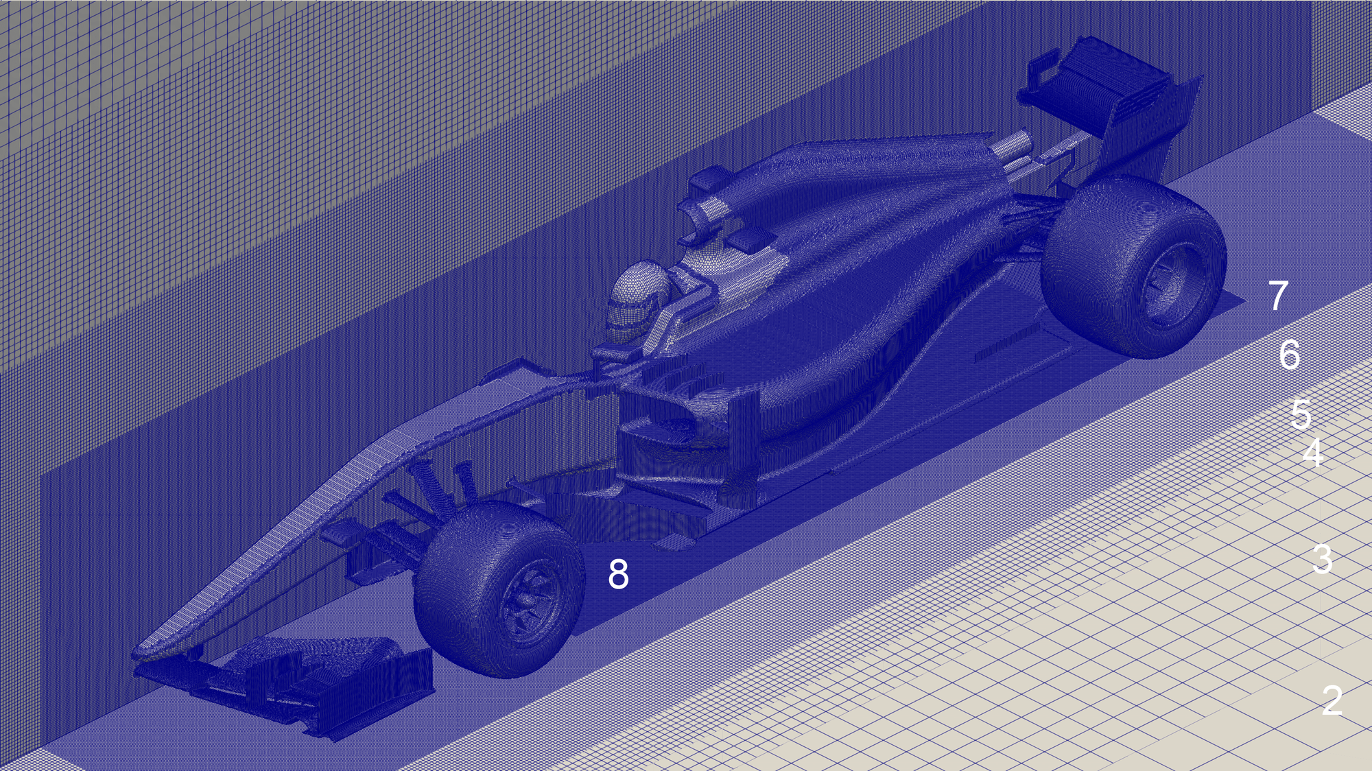
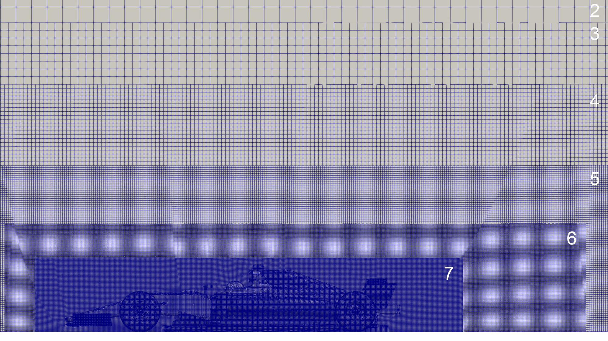
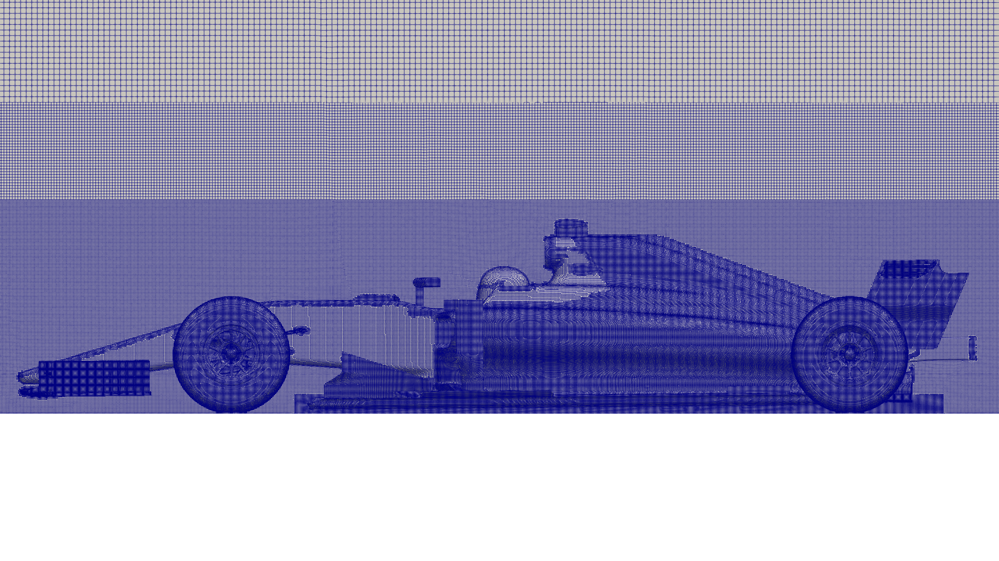
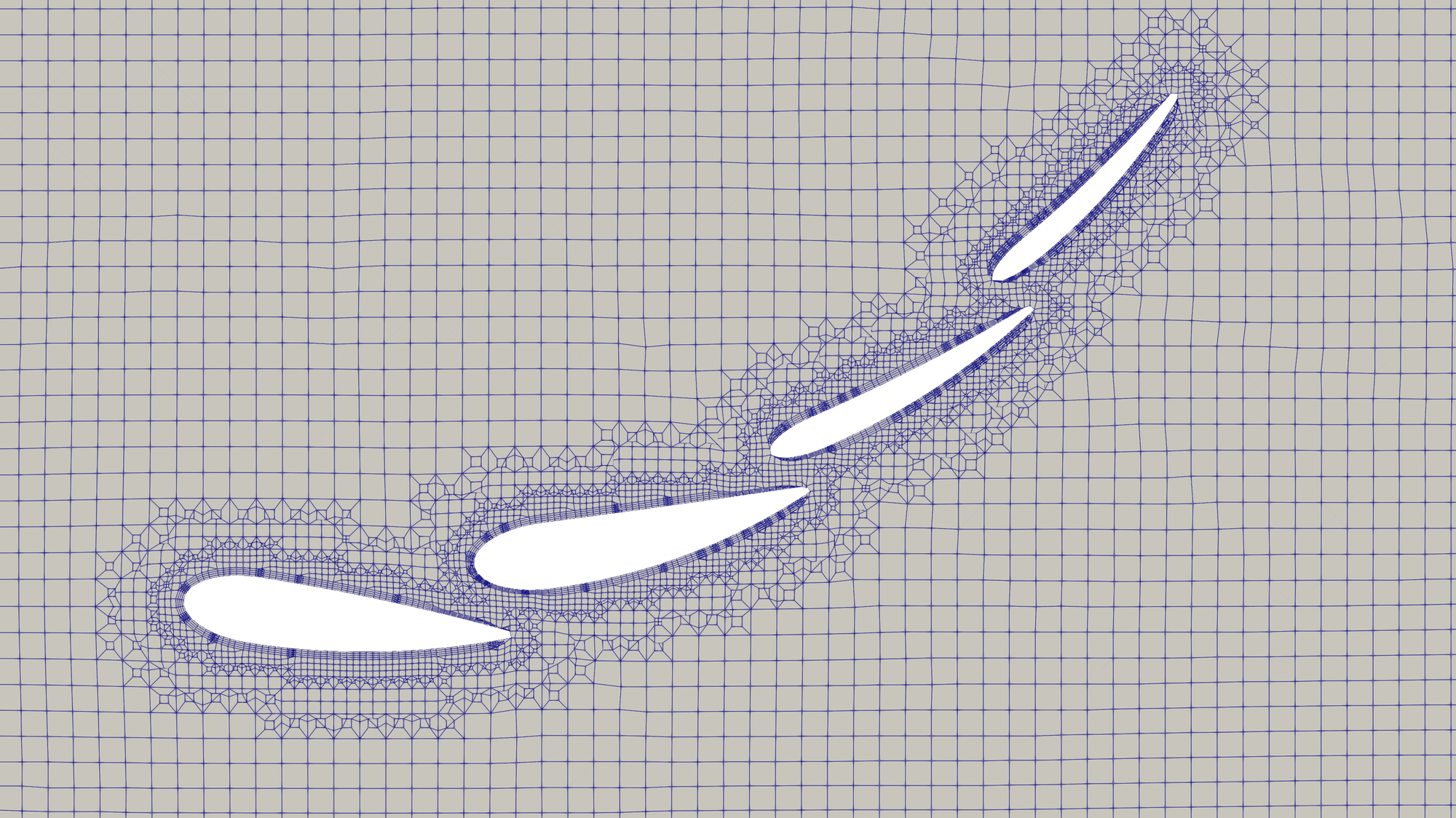
Due to the sensitivity to the complex flow structures involved in Formula one aerodynamics, it's important to produce a mesh with high surface resolution such that the shape of the geometry is resolved to a high standard. There are strong pressure and velocity gradients found around the car, including vortices that are important to capture, as they can have a large influence on what happens downstream. It's likely that mesh independency will not occur until meshes with cell counts over 100 million cells are reached. Unfortunately these cell counts are not possible on the hardware available, so results may not be mesh independent.
Due to hardware limitations, it was decided to only model half of the car. This ensures the geometry is resolved in the CFD mesh to be representative of the CAD model. Along with this, a fine mesh is required under the floor of the car, where there is little ground clearance. The underfloor contributes significantly to the downforce, so it's important to properly resolve the gap between the floor and ground plane. Wake refinement blocks have been used to capture this area under the car, and to generally control the volumetric refinement around the car.
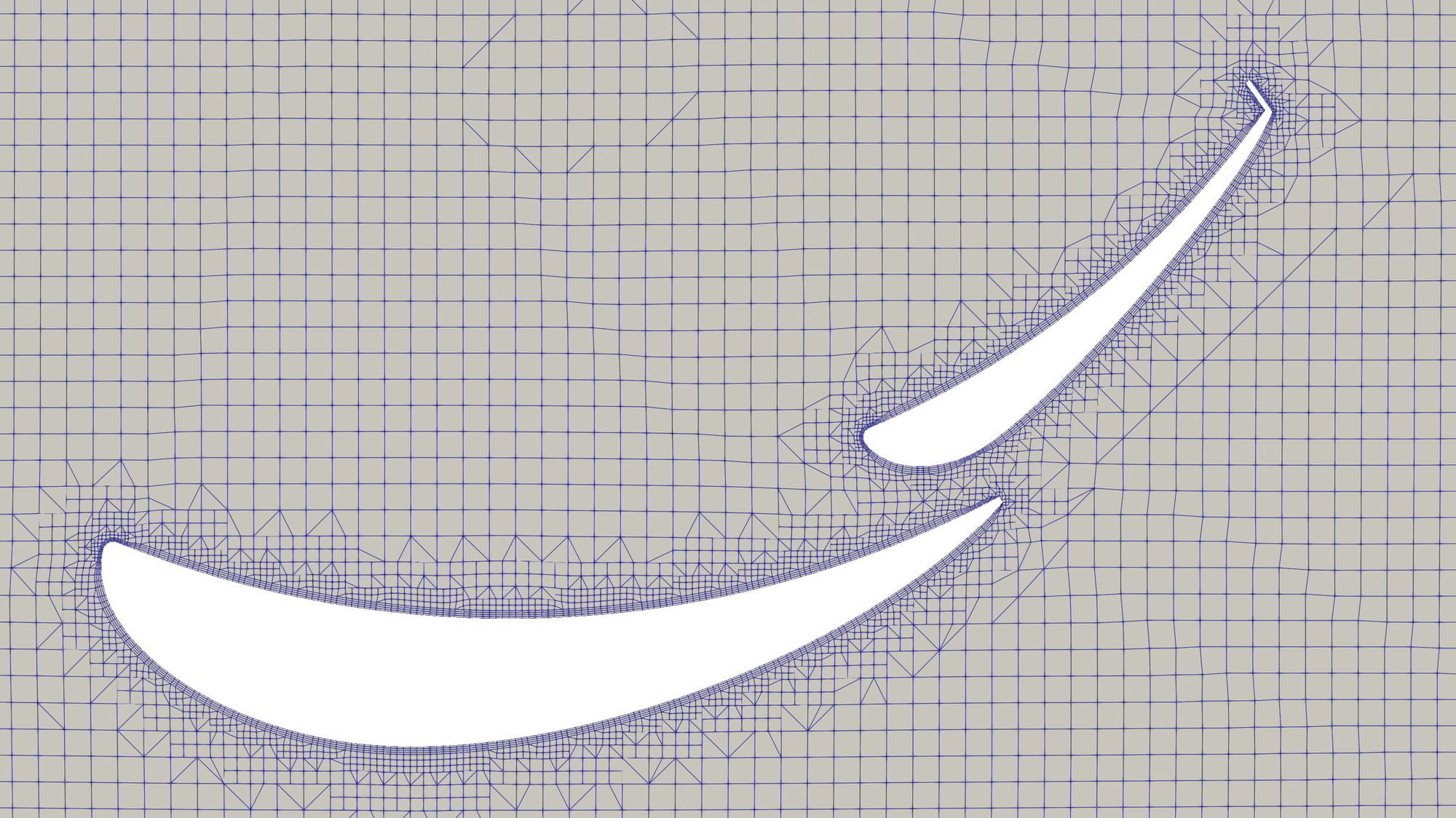
Wall functions have been employed to model the boundary layer. Most surfaces have 2 prism layers of equal thickness, set to x0.3 the local cell edge lengths. The front and rear wing have 4 prism layers.
There are numerous limitations to using a half-car approach. The first is that it can only be used for straight on flow conditions. It's impossible to model yaw, cross-wind or cornering flow conditions using a half-car approach. Another limitation is that the symmetry plane 'artificially' constrains the flow in the xz direction. This is less of a problem in the steady-state case, however for a transient approach, the wake should be free to oscillate in the y-direction and able to cross the symmetry plane.
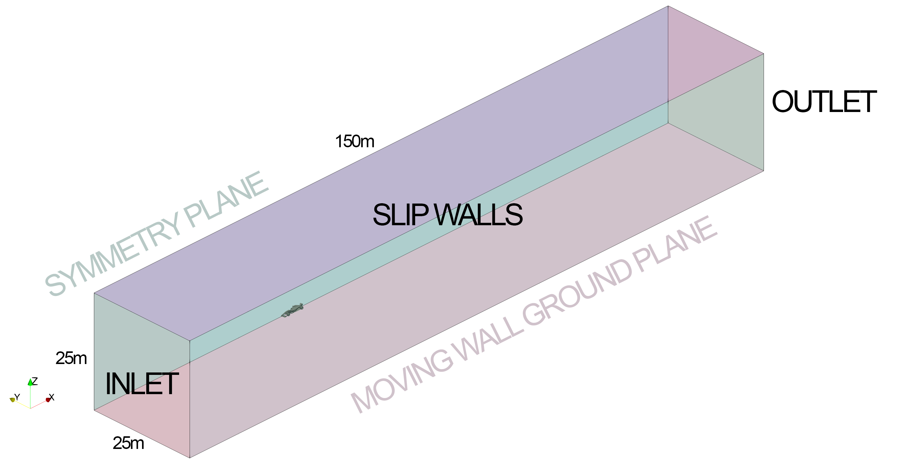
The car has been placed in a domain with dimensions 150m x 25m x 25m (x . y . z). The domain extends approximately 50m upstream of the car to the inlet, and 100m downstream to the outlet. These dimensions should ensure the blockage ratio between the car and the domain is minimal, and allows the wake to settle well before reaching the outlet.
Due to the limited time and computational resource for this project, a limited number of volume meshes were generated and a mesh sensitivity study was not feasible. The final mesh contained 39,981,943 cells and was accepted based on personal experience and best practices. The edge lengths of the hex cells correspond to the table below.
| cell level | 0 | 1 | 2 | 3 | 4 | 5 | 6 | 7 | 8 | 9 | 10 |
|---|---|---|---|---|---|---|---|---|---|---|---|
| edge length | 1 | 0.5 | 0.25 | 0.125 | 0.0625 | 0.0313 | 0.0156 | 0.0078 | 0.0039 | 0.0020 | 0.0010 |
The following video shows the mesh via a sweeping slice animation. The slice has been reflected in the y = 0m plane.
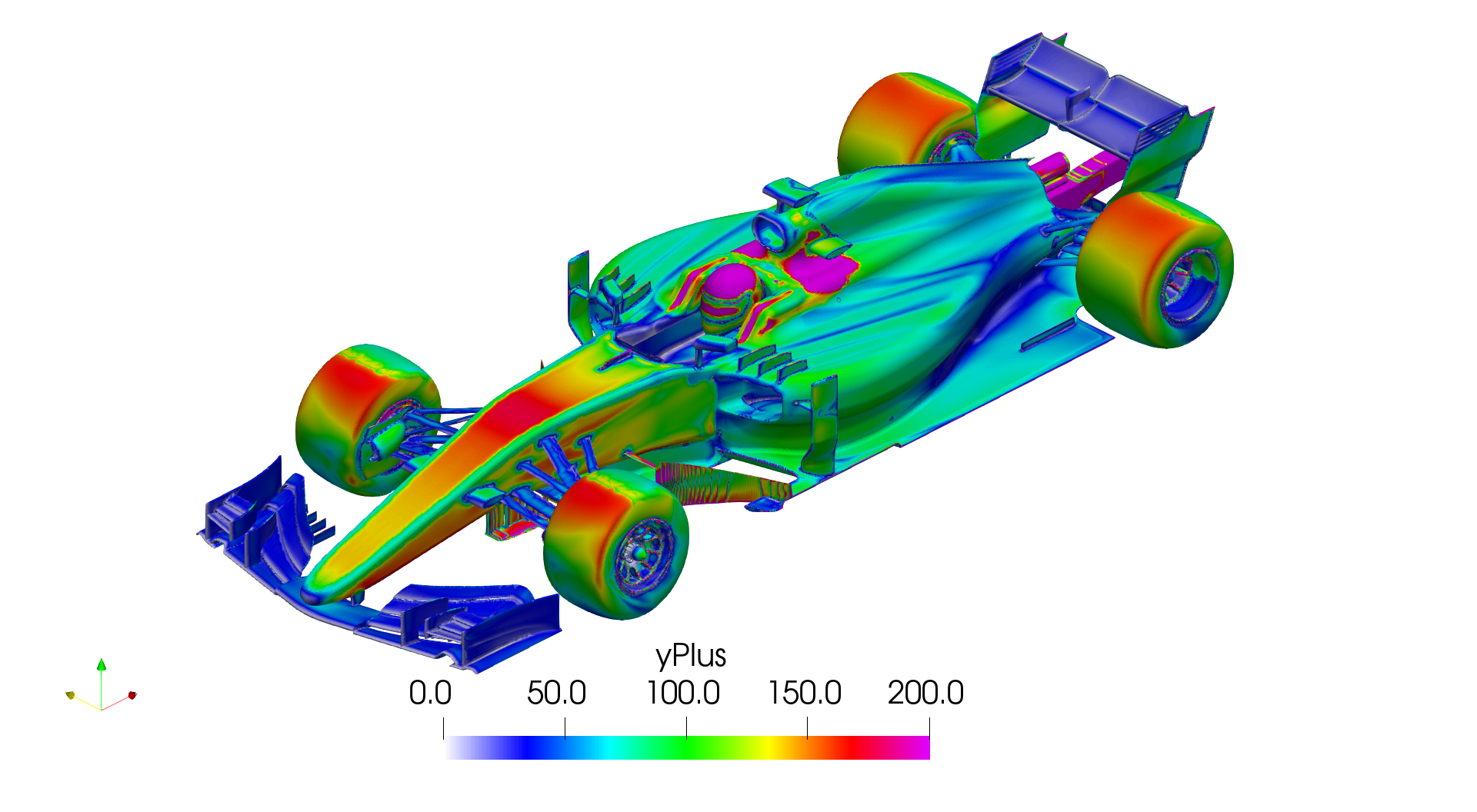
The y+ values at the car's surface are between 30-200 in most locations, as indicated on the plot below, produced from a RANS test case. The native OpenFOAM wall functions should provide a reasonable approximation of boundary layer profiles at these y+ values.
Methodology
The methodology followed for the CFD solve is summarised in the following points:
- Flow is treated as incompressible, isothermal and fully turbulent.
- Flow approaches at 0° yaw and a fixed, uniform velocity of 50m/s.
- Kinematic viscosity is fixed at 1.5E-05 m2/s.
- Density is fixed at 1.225kg/m3.
- A steady-state solution is resolved using the k-omega SST Reynold's Averaged Navier Stokes (RANS) turbulence model and the simpleFoam solver.
- The solution is resolved for 1000 iterations, before forces and field variables are averaged over a further 500 iterations.
- Transient solution is resolved using the k-omega SST Delayed Detached Eddy Simulation (DDES) turbulence model and the pisoFoam solver.
- The DDES solution is initialised from 1000 RANS iterations, then run for 1.5s of physical time using a 0.0005s timestep. Forces are averaged over the final second and field variables are averaged over the final 0.5s.
- Wheel rotation is modelled using a moving wall boundary condition on the tyres, rims and other rotating components.
- The rotation of the spokes is modelled using an MRF approach.
- A moving wall boundary condition is employed on the ground plane, matching the flow speed (50m/s).
- No brake disk modelling.
- Radiators are modelled using a porous region, following a Dary Forchheimer methodology
- Air intake and exhaust flow modelled using a fixed volumetric flow rate inlet and outlet
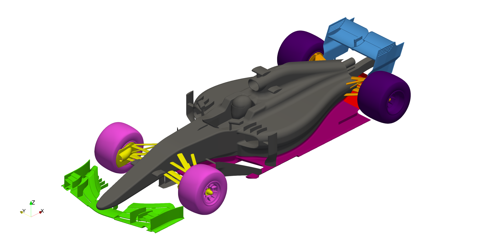
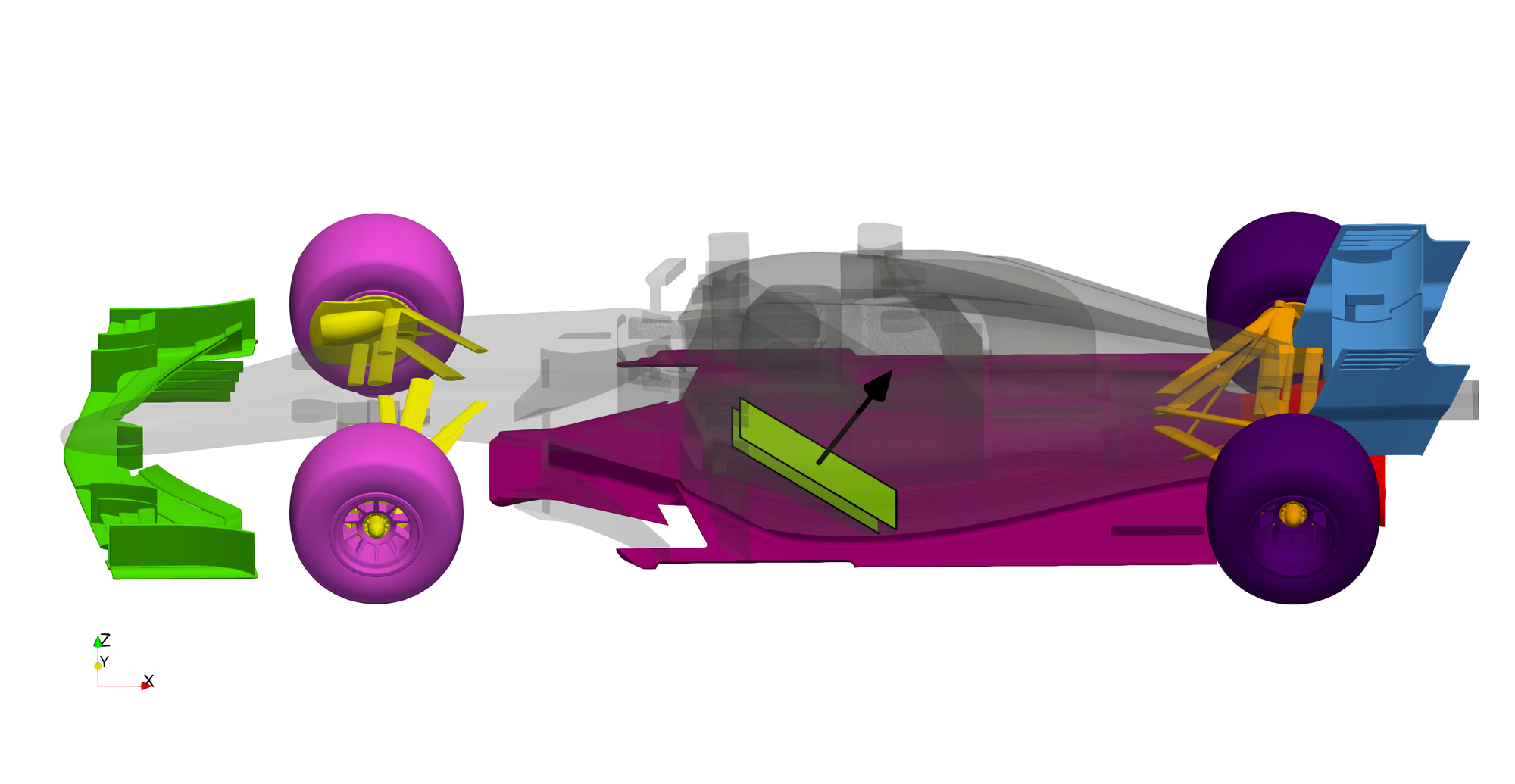
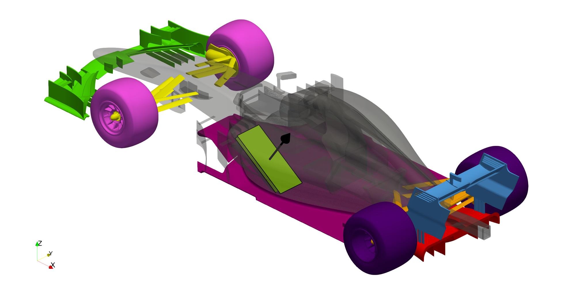
An additional surface was added to the model to define the cellZone in which the MRF approach is applied. This surface encompassed the rim spokes and is shown in green below. Another image is presented showing the moving wall boundary condition applied to the wheels; A velocity magnitude and a z-velocity image are shown, as a check wheel omega was calculated correctly and tyre rotation is applied in the correct direction.
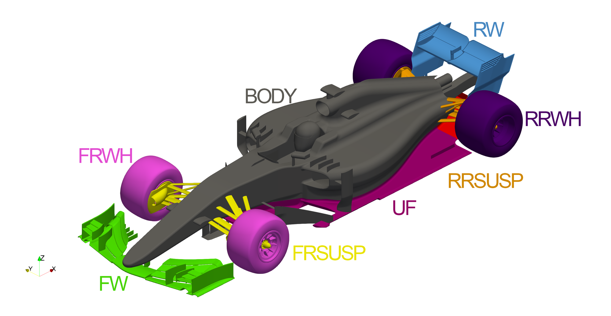
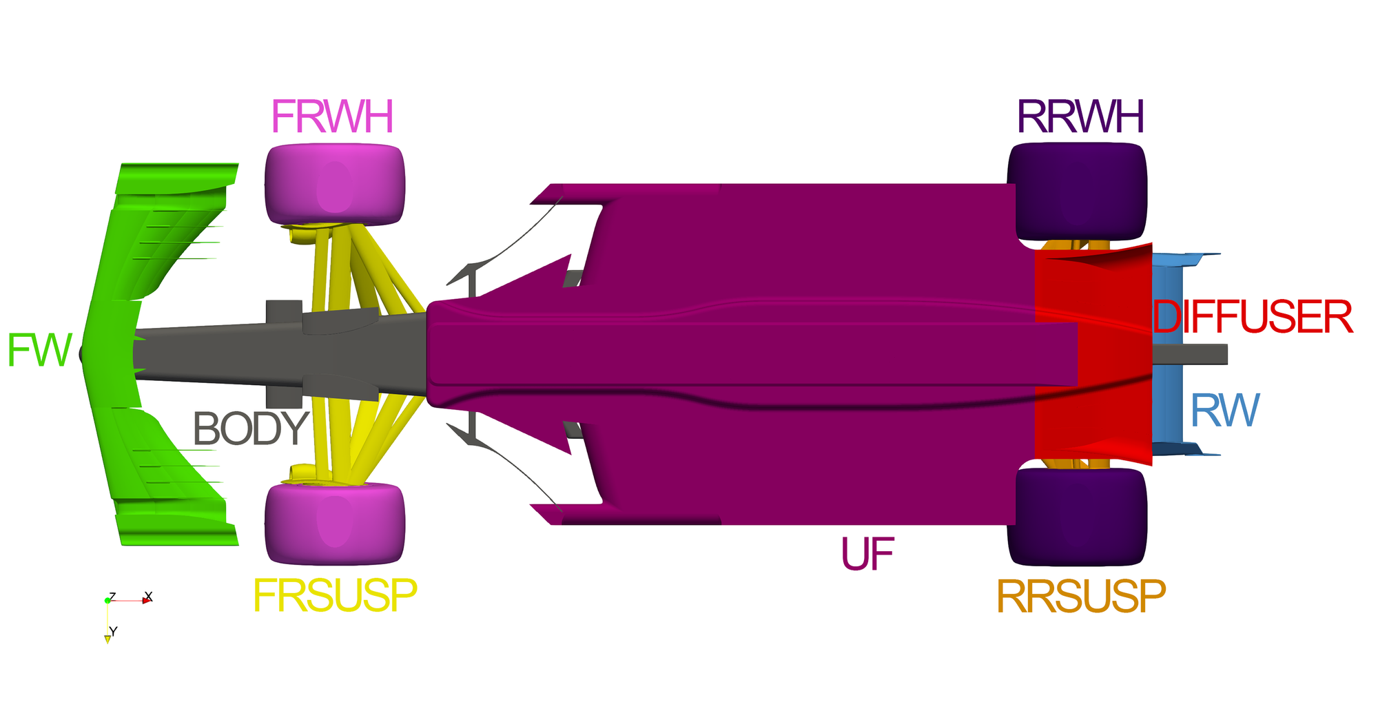
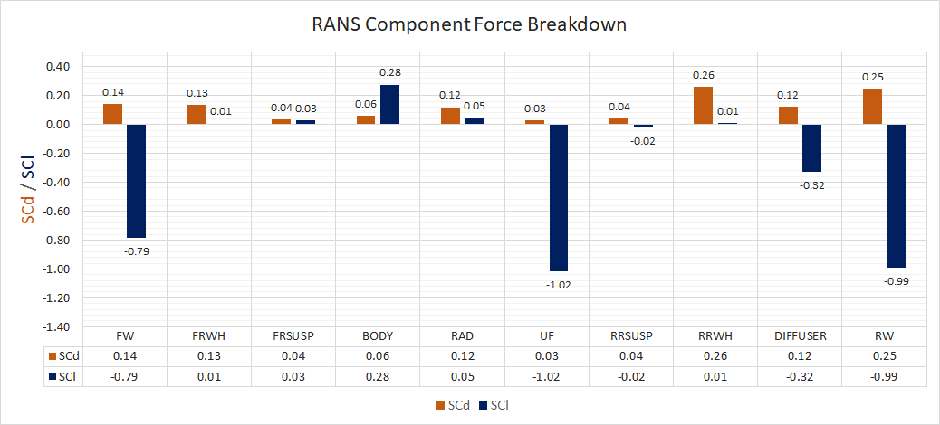
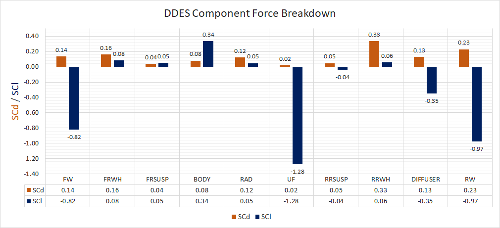
The car has been split up into multiple force groups, to gain a better understanding of how the drag and lift forces are distributed around the car. These force groups can be seen below. The radiator housing is within the 'BODY' group, however the 'force' imparted on the car from the porous zone is reported as a separate 'RAD' group. All components within the engine bay are also grouped into the 'BODY' group, including the geometry representing the engine.
The radiator has been modelled by creating a cellZone bounded by two existing planes within the radiator housing. The pressure loss through this porous zone is governed by the following equation:
\[ ΔP = µ\:L\:U\:d + \frac{1}{2}\:ρ\:L\:U^2\:f \]
where:
ΔP = Pressure loss (Pa)
µ = Dynamic viscosity of the fluid (kg/ms)
L = Thickness (m)
U = Fluid velocity (m/s)
ρ = Fluid density (kg/m3)
d = Darcy coefficient
f = Forchheimer coefficient
The Darcy and Forchheimer coefficients can be derived experimentally by measuring the pressure drop through the radiator under known conditions and using a curve fitting approach. For the purposes of this project, d and f have been set to 4.0E7 and 100 respectively in the normal direction (through the radiator). Values in the perpendicular directions have been set sufficiently high, ensuring the flow is constrained in the normal direction through the radiator. These values could be far from reality for a typical F1 radiator.
Monitors were setup on the inlet and outlet faceZones of the radiator, which reported area-weighted average pressure, velocity and total pressure. This allows for an extra check of convergence to ensure pressures and flow rates through the radiators have stabilised and also provides a measure for the overall pressure loss through the radiator.
Results
Steady State RANS Forces
The steady-state k-omega SST RANS case was run for 1000 iterations, at which point the forces were deemed to have stabilised. The flow field and forces were then averaged over a further 500 iterations. The force convergence on all components excluding the radiator is presented, along with a moving average starting from iteration 1000.
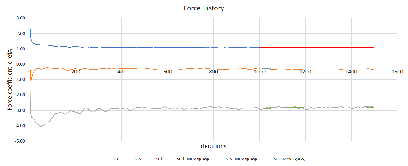
Forces have been nondimensionalised by the freestream dynamic pressure and left in a Force coefficient x reference Area (SCd/SCl) format.
\[ SCd = \frac{Drag\:(N)}{\frac{1}{2}\:ρ\:U_\infty^2} \]
\[ SCl = \frac{Lift\:(N)}{\frac{1}{2}\:ρ\:U_\infty^2} \]
In these equations, Drag and Lift represent the positive force in the x and z direction (from the coordinate system indicated on the force group images). All forces have been multiplied by 2 before nondimensionalisation, to account for the other side of the modelled half-car. The total forces acting on the car are presented in the table below. The Aerodynamic efficiency is also presented, as -SCl/SCd along with the front balance (percentage of downforce acting through the front axel). Note, negative lift indicates downforce.
| RANS TOTAL FORCE (FULL CAR) |
|---|
| SCd |
| 1.20 |
| SCl |
| -2.77 |
| AERODYNAMIC EFFICIENCY |
| 2.30 |
| BALANCE |
| 38.9% |
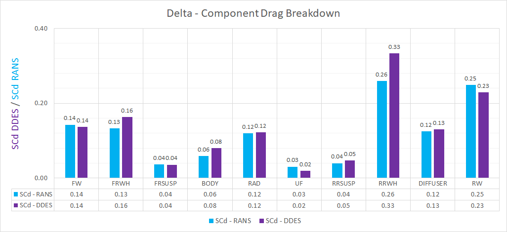
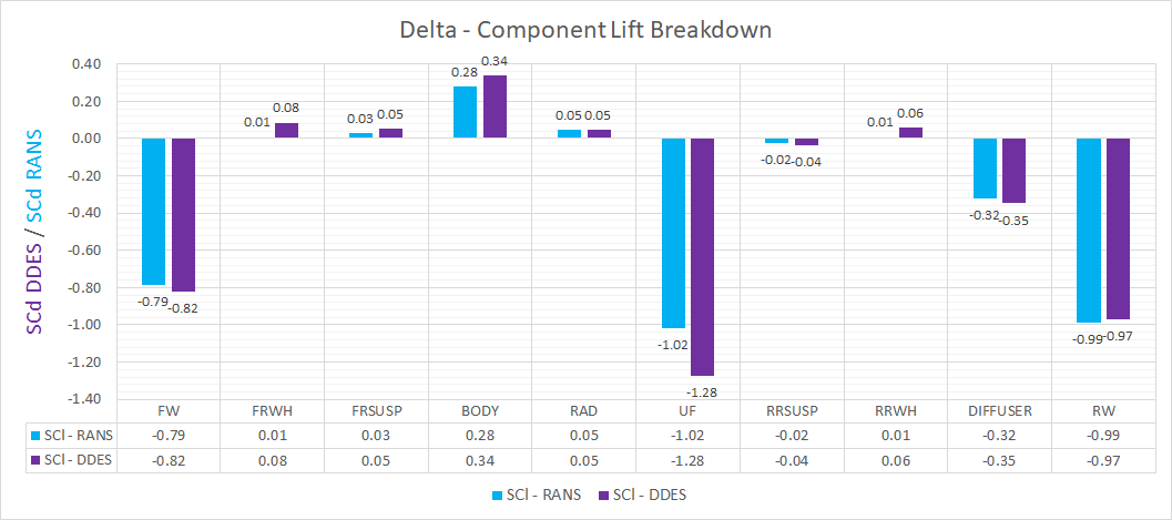
The component contributions to the overall forces are indicated below.
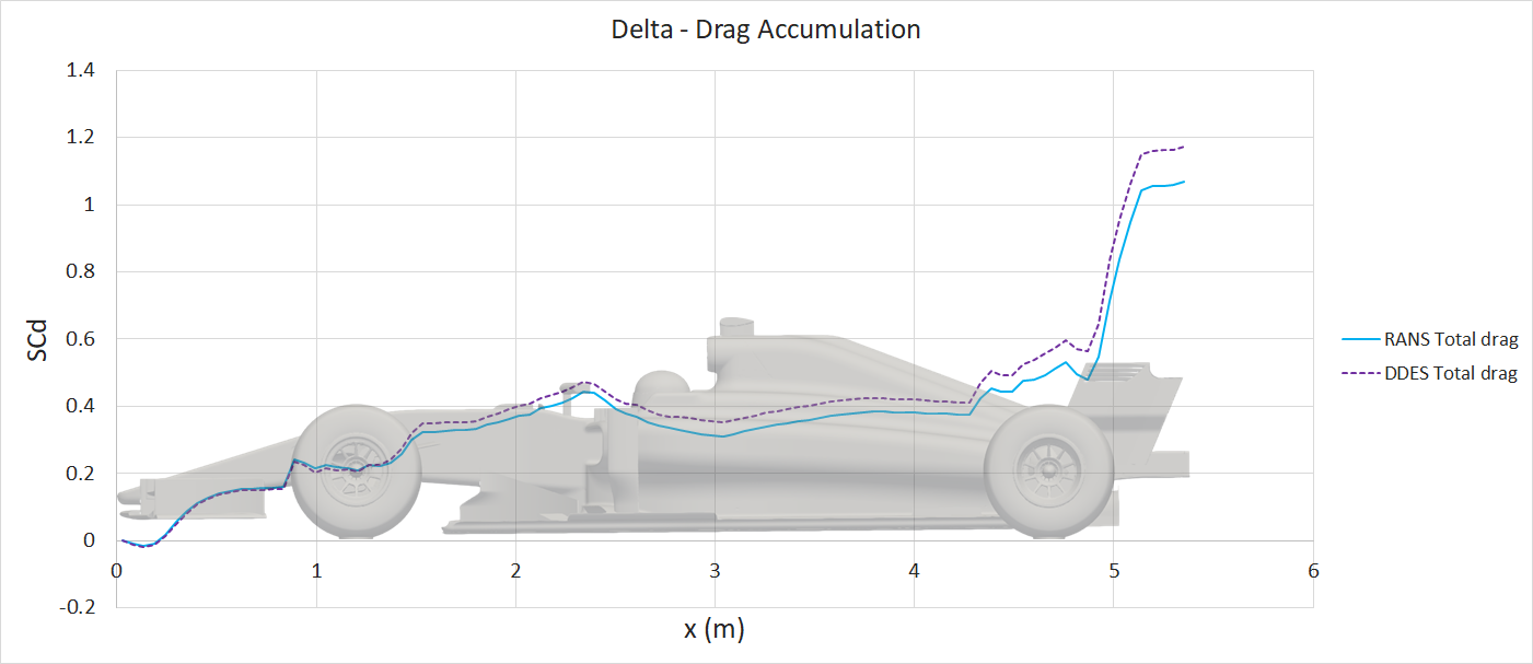
A more interesting way to visualise the component force contributions is to look at the force distribution and accumulation over the car's length. There doesn't seem to be an easy way to calculate this directly in OpenFOAM, however it is relatively straight forward in Paraview with some simple code. The following steps outline the methodology used to extract longitudinal force data.
- Write out all vehicle surfaces using a functionObject, ensuring the pMean scalar (iteration/time averaged static pressure) and WallShearStressMean vector on the surfaces are inlcuded.
- Read surface file into paraview, extract dimensions (specifically xmin and xmax).
- Add a paraview calculator to dot product pMean with the local normal unit vectors (calculating the surface pressure contribution in each direction depending on face orientation).
- Divide the car into 100 discretised sections.
- March through the 100 sections, applying an integrate variables filter at each discretised section and writing out the result to a csv file. This filter just multiplies field variables by local face areas and sums the results for the entire section.
- Calculate the x-position of the section center and write the result to a separate file.
- Run a simple bash script to concatanate the force data .csv files into a single file.
- Import the final data into excel and process the raw data into distribution and accumulation.
Interestingly, the WallShearStress vectors written out by OpenFOAM appear to be the shear stresses acting on the fluid, not the car. This was simple to correct in Paraview by inversing the sign (WallShearStress*-1). Overall, the methodology described above was very fast to run, however RAD (porous zone) forces are not accounted for.
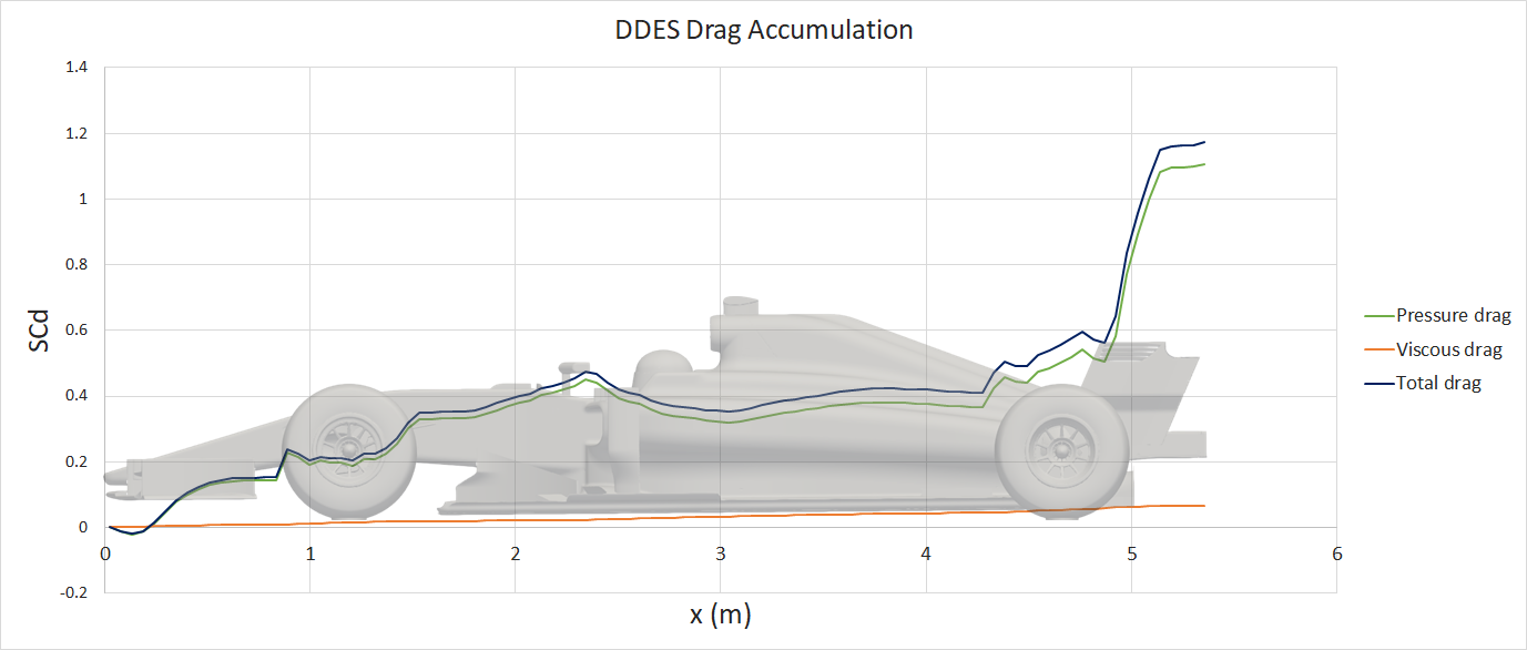
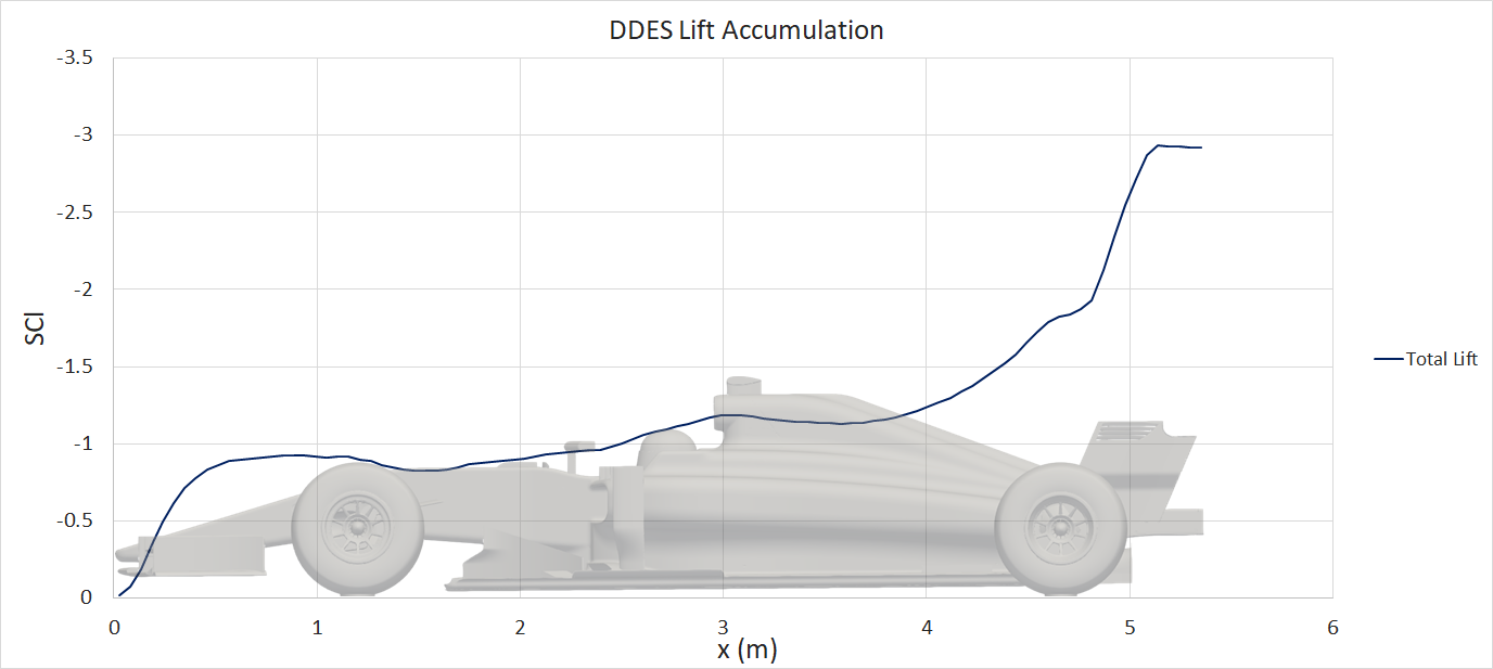
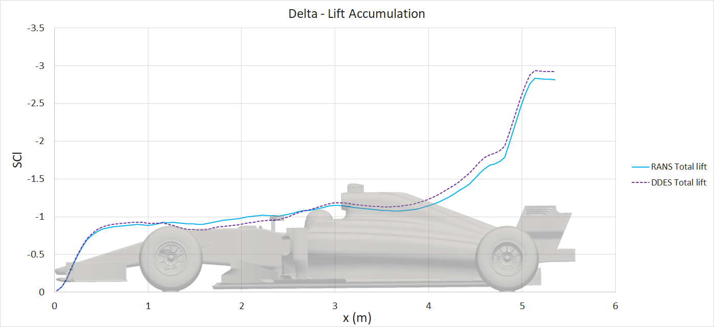
The resulting iteration averaged steady-state RANS force accumulation plots are presented:
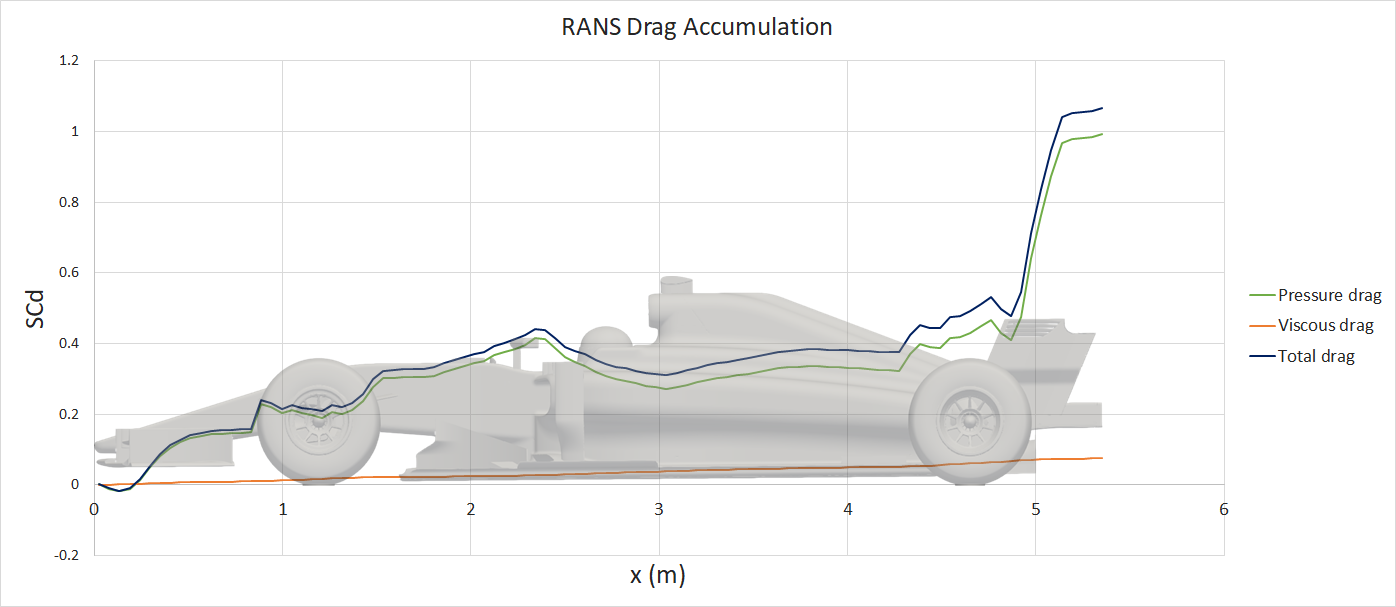
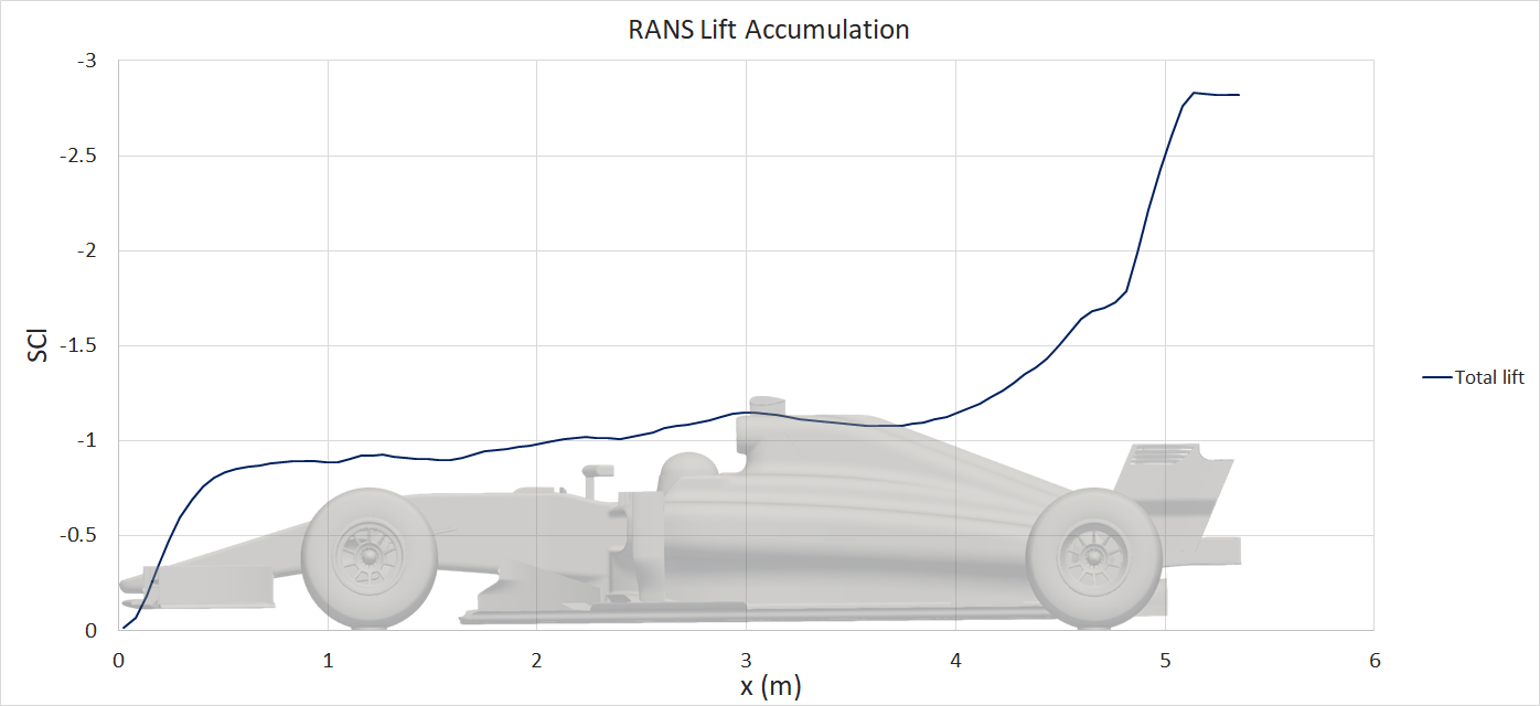
The pressure and viscous drag contributions are plotted for the drag accumulation, however there are minimal viscous forces acting in the lift direction, hence only the total lift has been plotted.
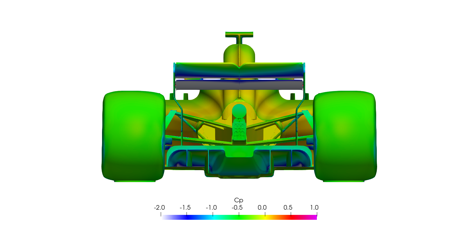
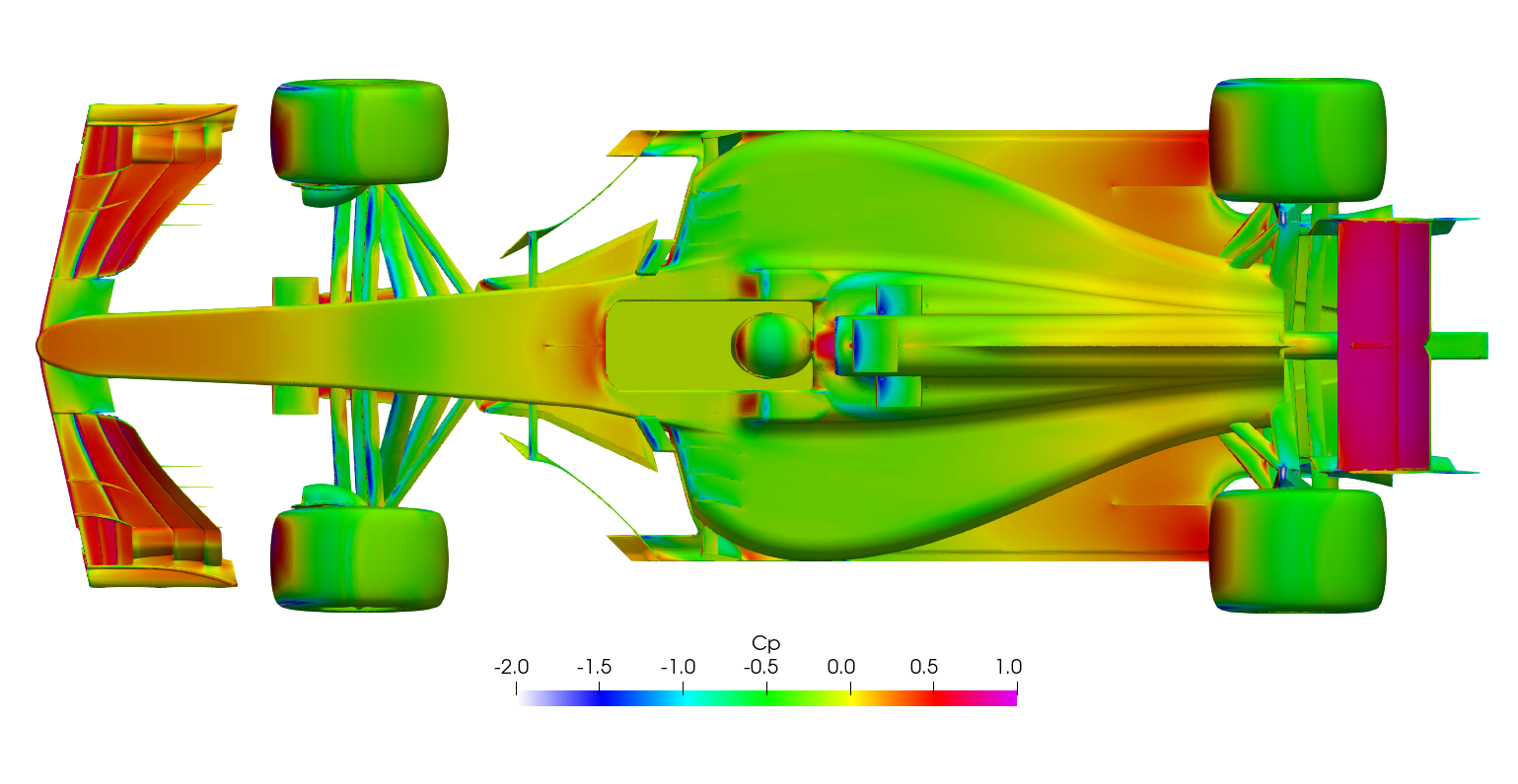
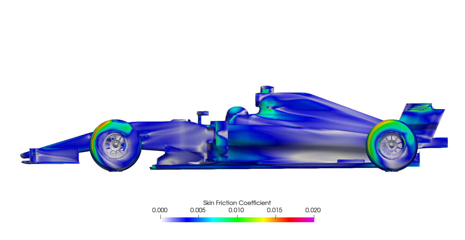
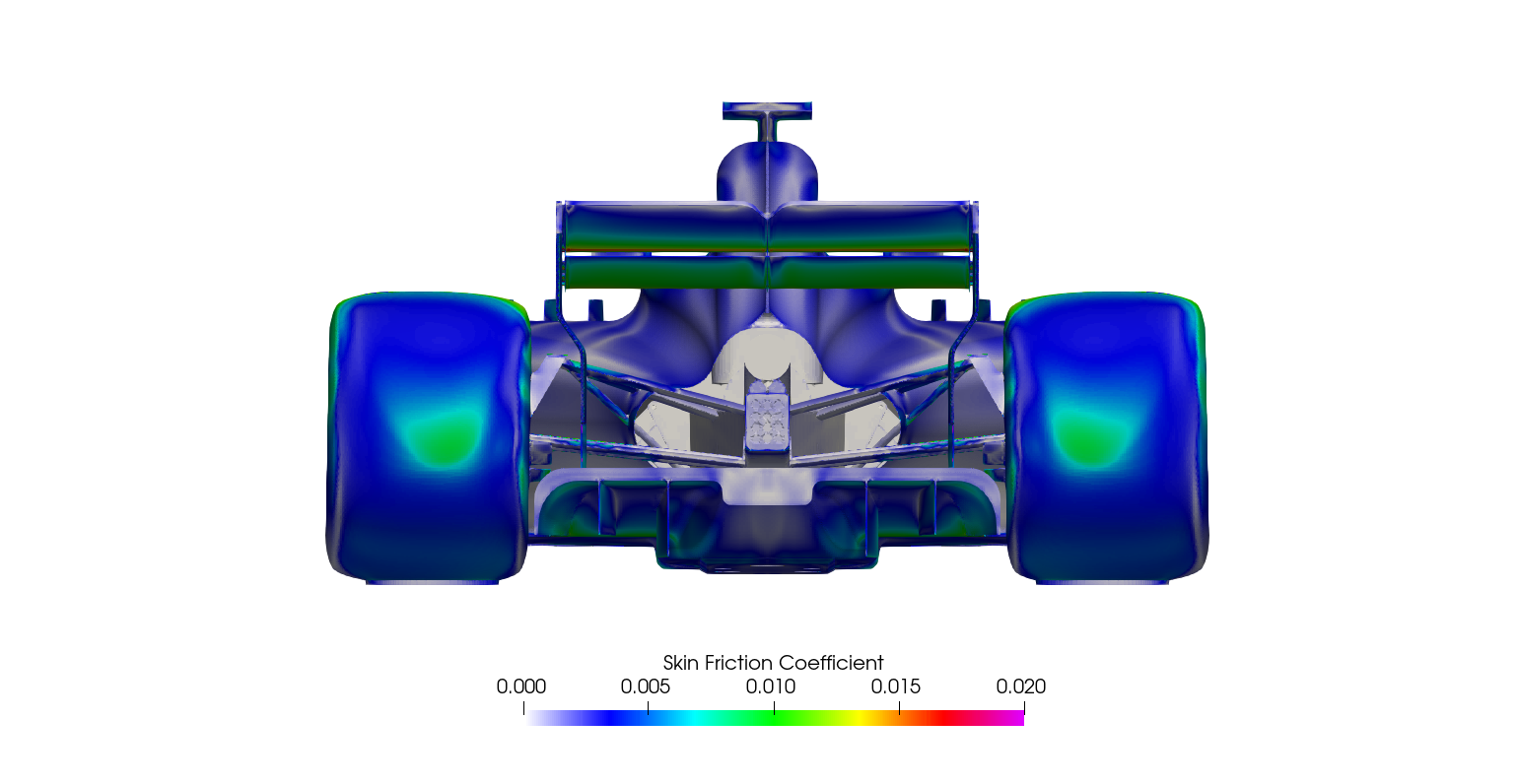
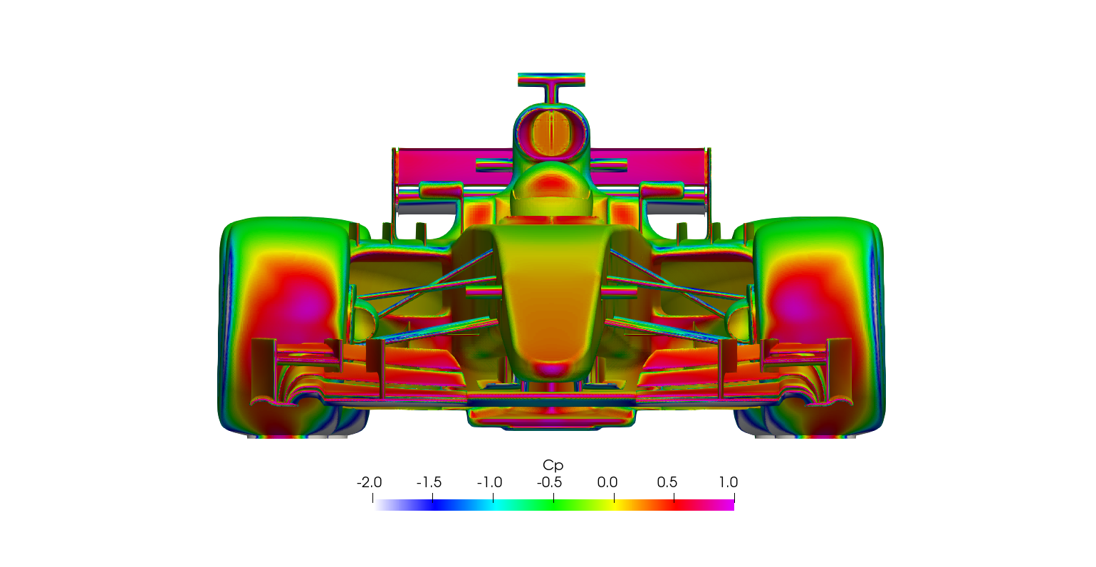
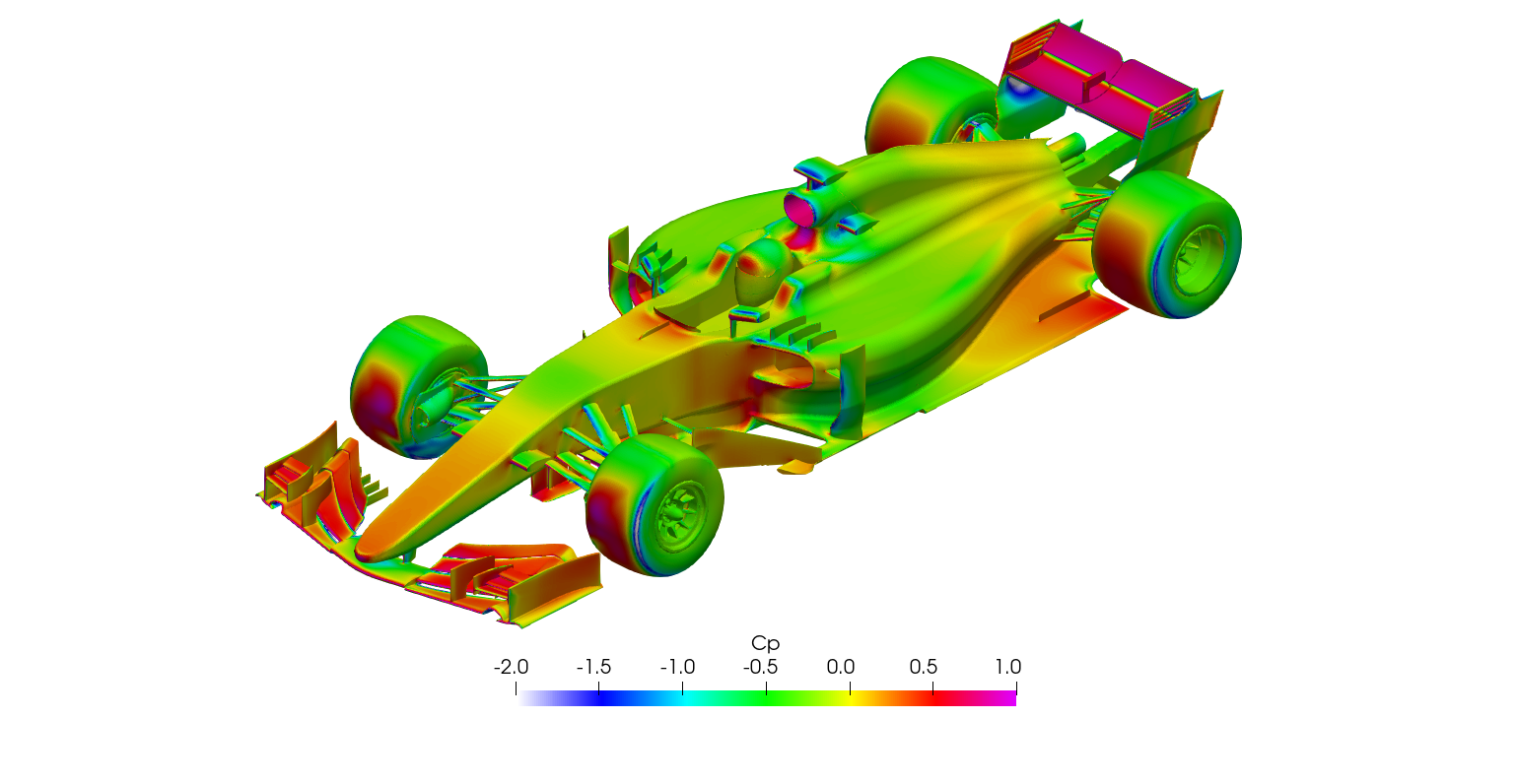
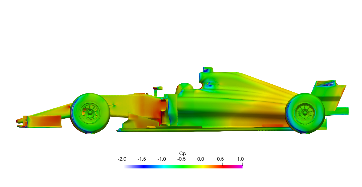
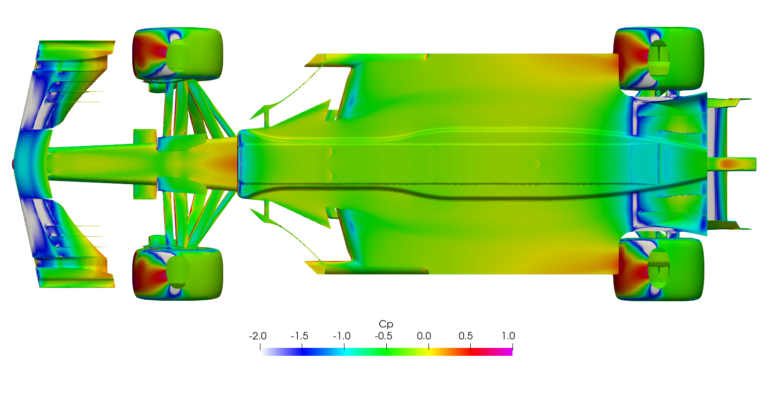
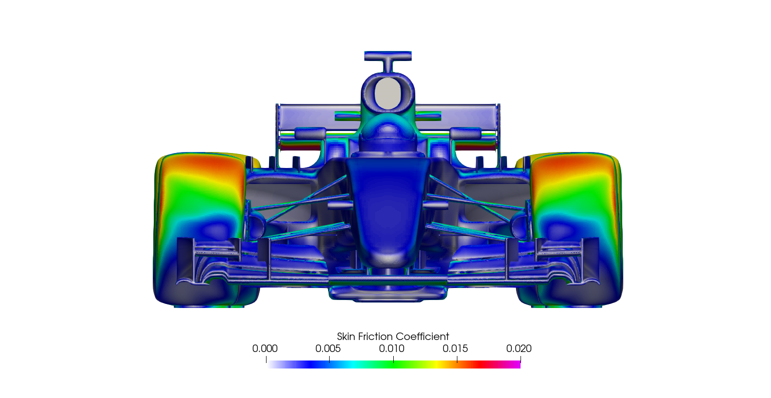
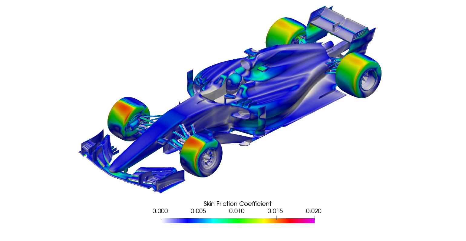
Steady-state RANS Post-processing
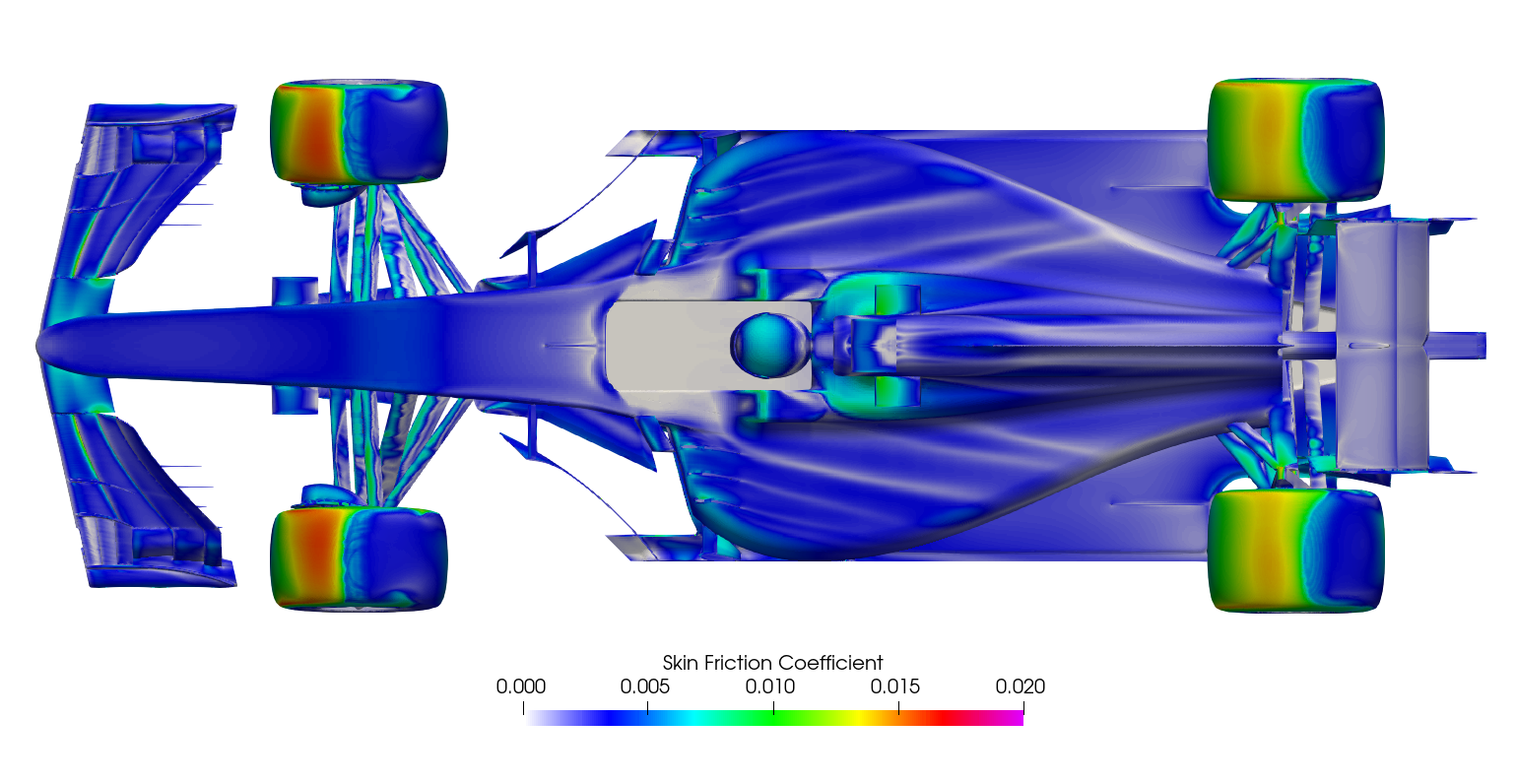
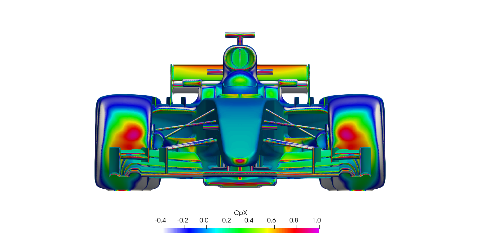
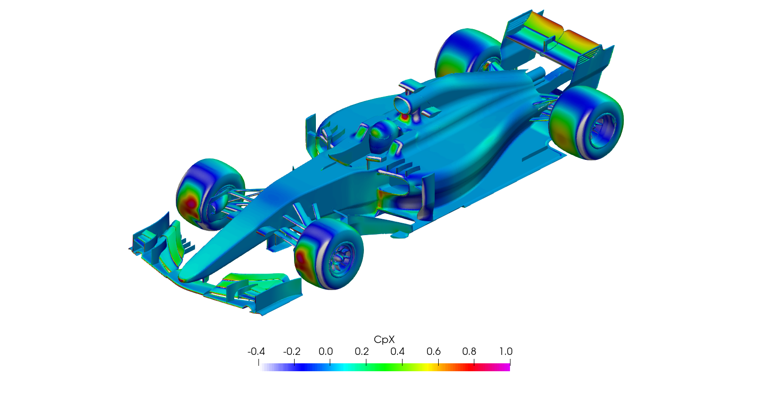
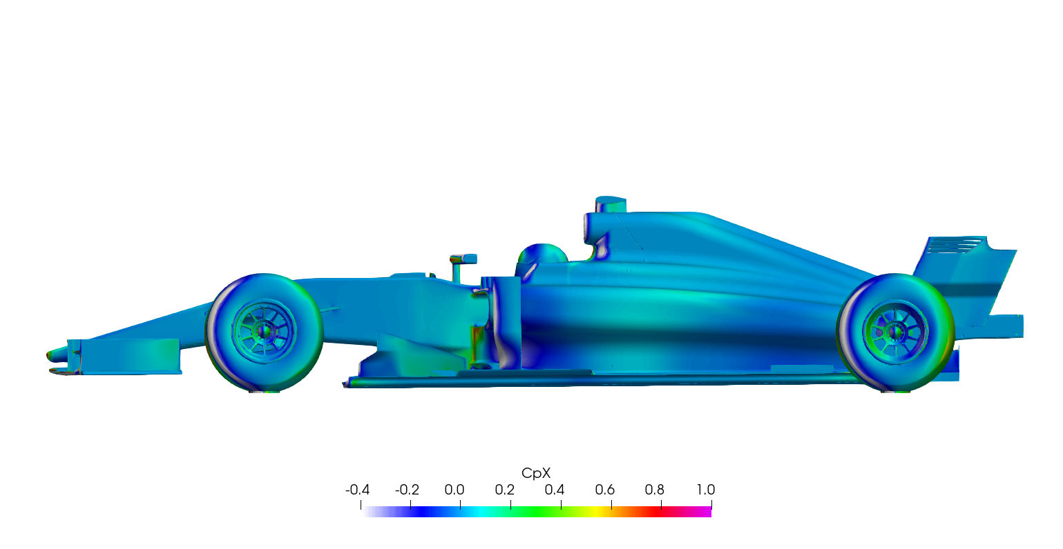
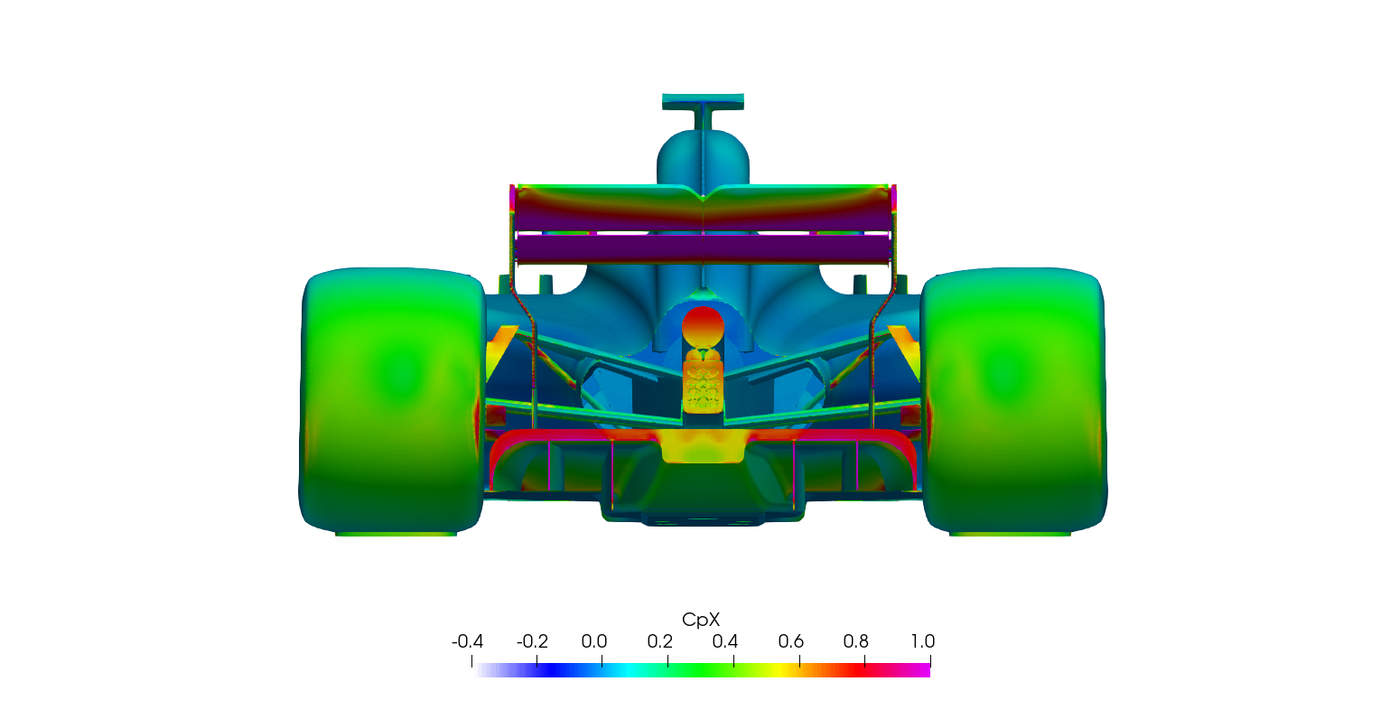
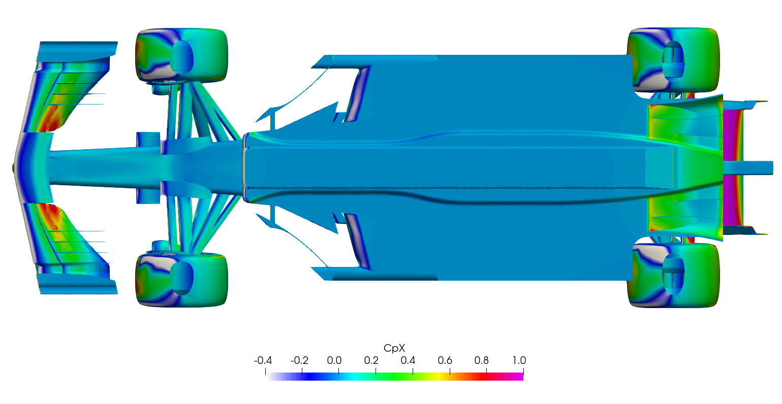
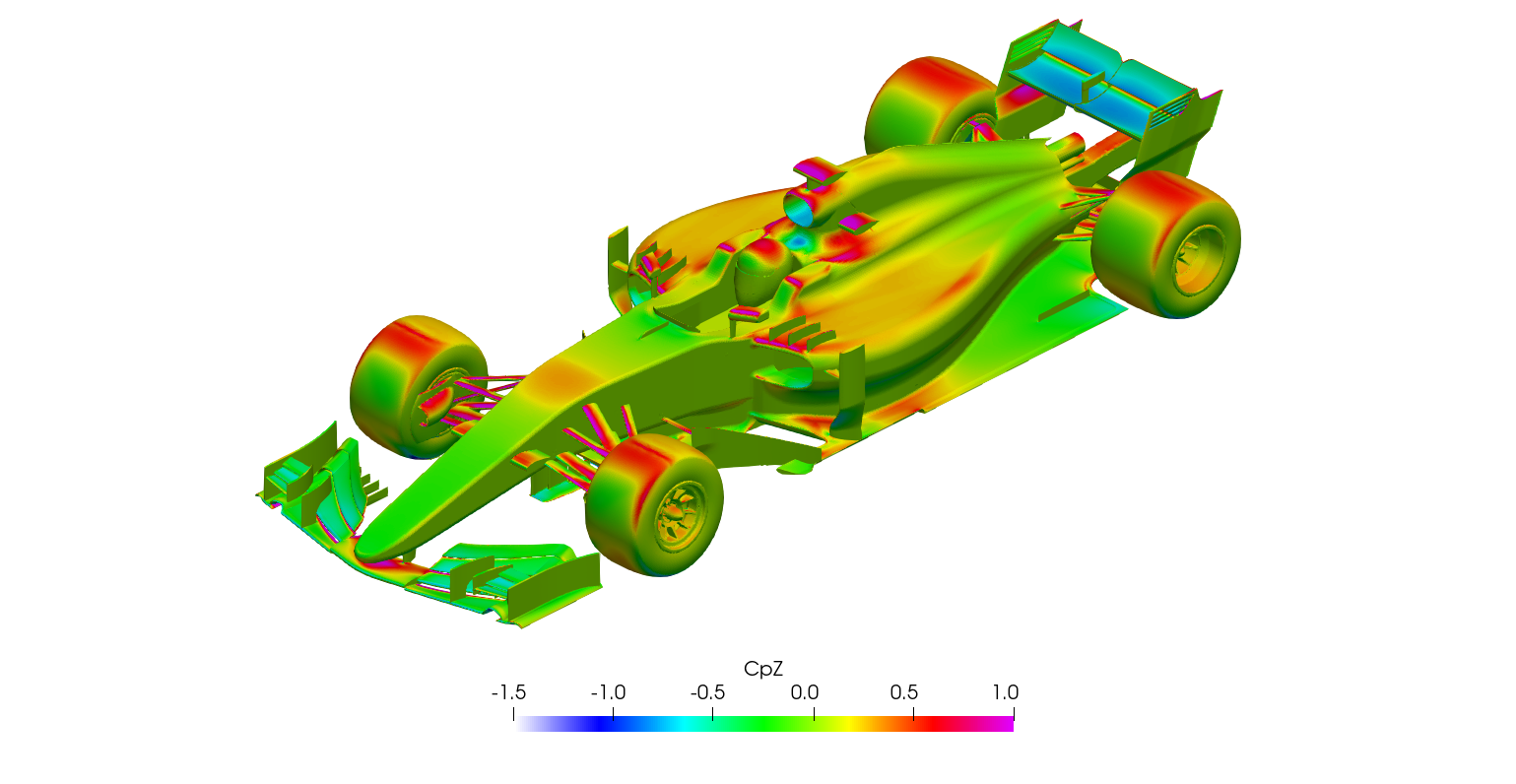
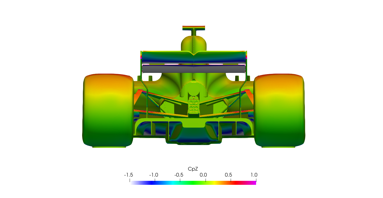
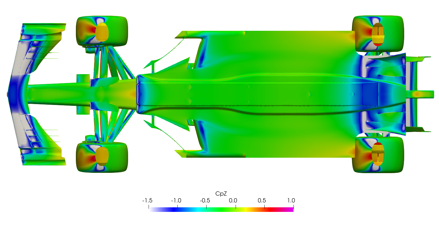
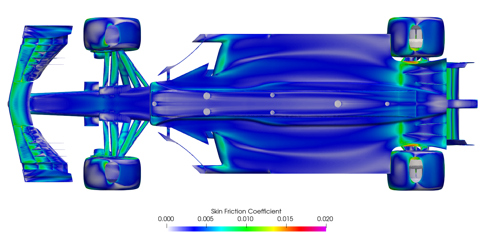
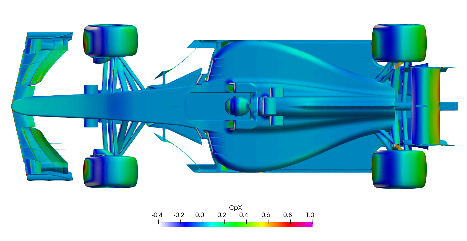
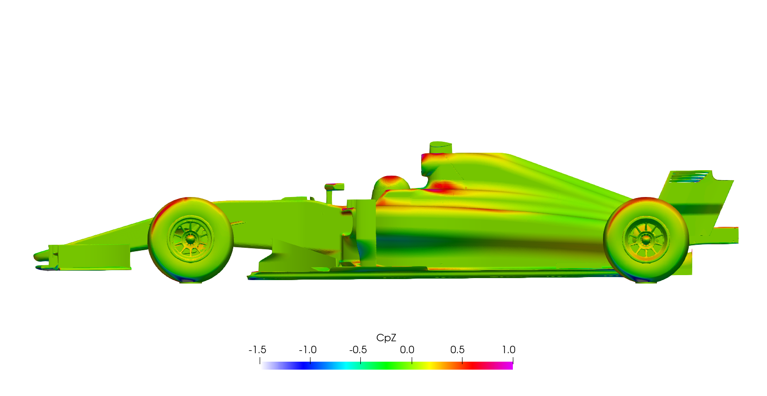
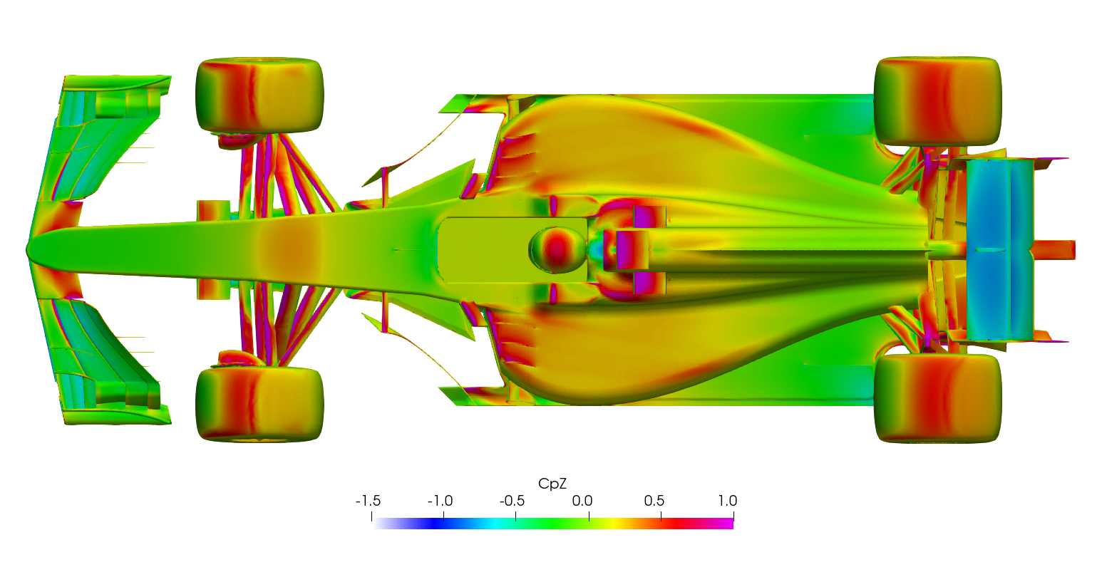
Surface plots for a range of field variables are presented for the reader to browse at leisure. These images provide further insight into how the forces are manifested, highlighting areas/components experiencing high/low surface pressures and shear stresses. It's important to include the face orientation when considering the effect of the pressure at the surface, hence pressure is often presented in terms of CpX (drag direction) and CpZ (lift direction). This is calculated by multiplying the static pressure coefficient by the directional component of the face normal unit vector. Wall shear stress is also presented as skin friction coefficient. This is often used in conjunction with near wall velocity to indicate the flow energy close to the surface, highlighting any areas where the flow is weakly attached, or separated. In summary:
\[ Cp = \frac{static\: pressure}{\frac{1}{2}\:ρ\:U_\infty^2} \]
\[ Cf = \frac{Wall\:Shear\:Stress}{\frac{1}{2}\:ρ\:U_\infty^2} \]
\[ CpX = \frac{static\: pressure\:\times\:x-component\:of\:face\:normal}{\frac{1}{2}\:ρ\:U_\infty^2} \]
\[ CpZ = \frac{static\: pressure\:\times\:z-component\:of\:face\:normal}{\frac{1}{2}\:ρ\:U_\infty^2} \]


Transient DDES Forces
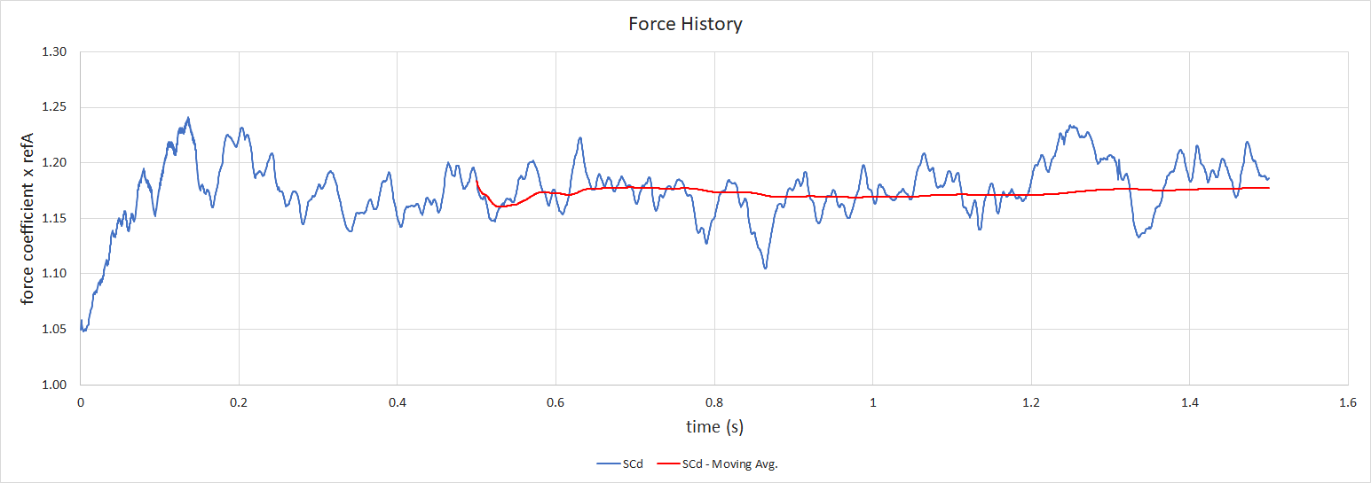
The transient half-car simulation was run for a total of 1.5 seconds of physical time, using a 0.0005s timestep. The transient simulation was initialised using the steady-state result, after 1000 iterations. Forces were averaged from 0.5s to 1.5s and field variables were averaged between 1.0s to 1.5s.
As previously mentioned, running a half-model transiently is typically avoided, since the wake should be free to move in the y-direction, which the symmetry plane prevents. However, one of the goals of this project from the outset was to establish a steady RANS and transient DES methodology in native OpenFOAM, thus the transient half-car case was created. This is a very large approximation and will likely effect the results significantly, especially near the symmetry plane. Nonetheless the results are presented.
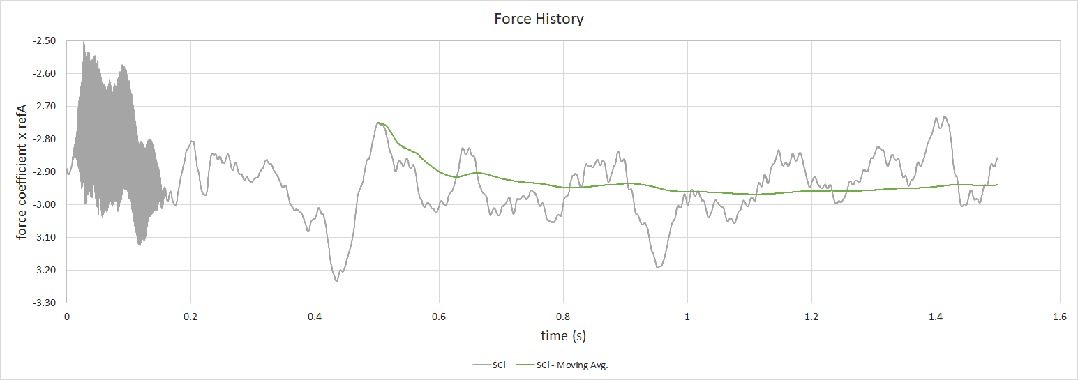
First of all, the force traces. During the first 0.25 seconds, the simulation suffered numerical instability. This was initially spotted in the force traces, showing up as a large fluctuation in lift. This was fixed by modifying the schemes. The case was still in a reasonably suitable position to run-on, without the need to restart. The resulting force traces for Drag and Lift are shown below.
The time-averaged forces, component contributions and force accumulation plots are presented similarly to the steady-state results.
| DDES TOTAL FORCE (FULL CAR) |
|---|
| SCd |
| 1.31 |
| SCl |
| -2.87 |
| AERODYNAMIC EFFICIENCY |
| 2.20 |
| BALANCE |
| 38.0% |
Transient DDES Post-processing
The surface plots for the time-averaged DDES results are presented for browsing.


Steady-state RANS vs. Transient DDES
There are differences in force predictions between the RANS and DDES approaches. The RANS result is a steady-state solution, meaning the time-varying flow features are not resolved. RANS cases are significantly 'cheaper' to compute, due to the reduced solve times, but generally struggle to provide an accurate prediction when bluff-bodies and large separated regions are present within the solution.
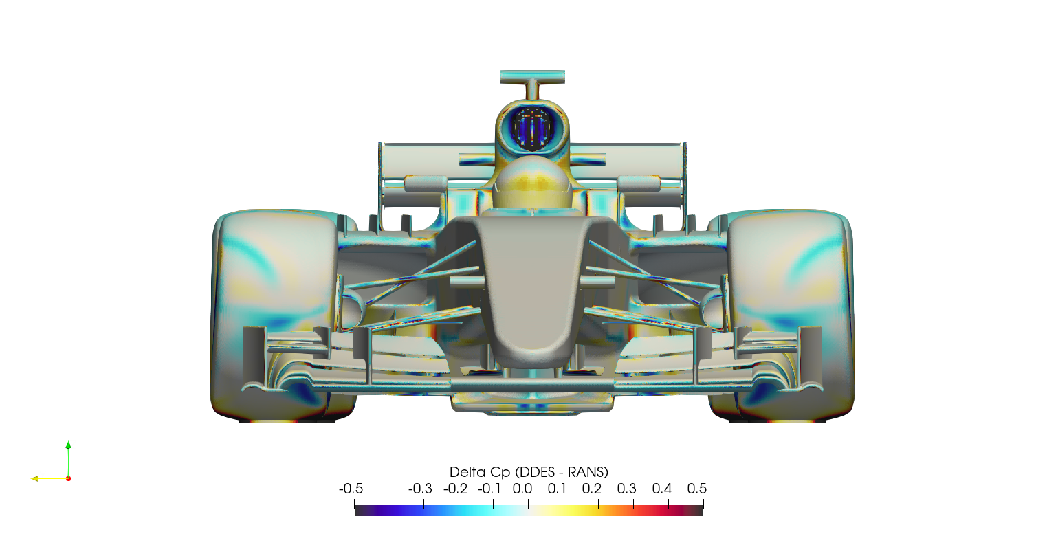
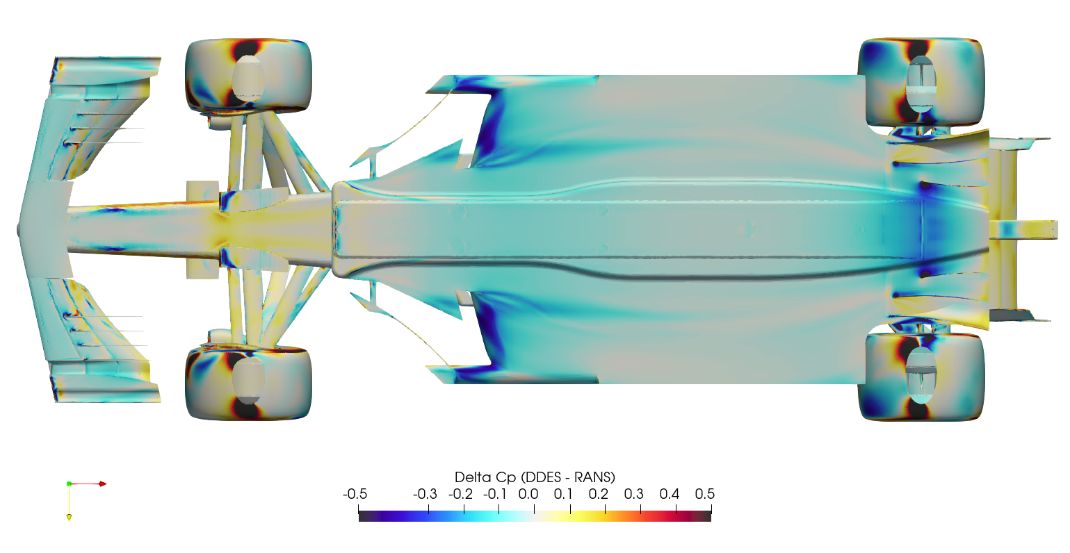
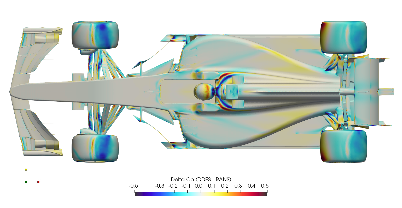
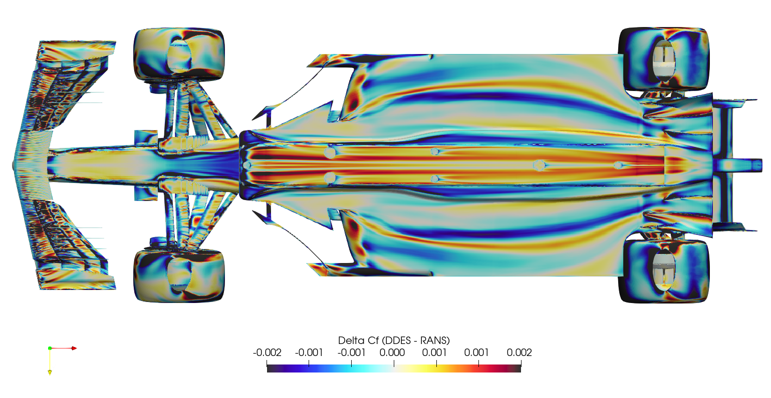
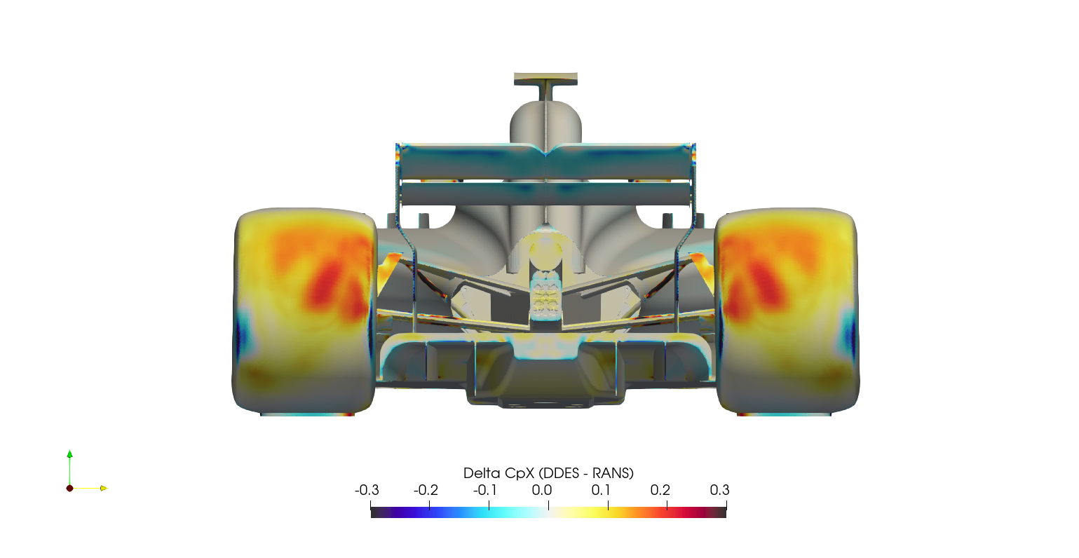
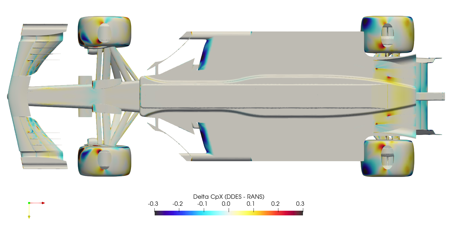
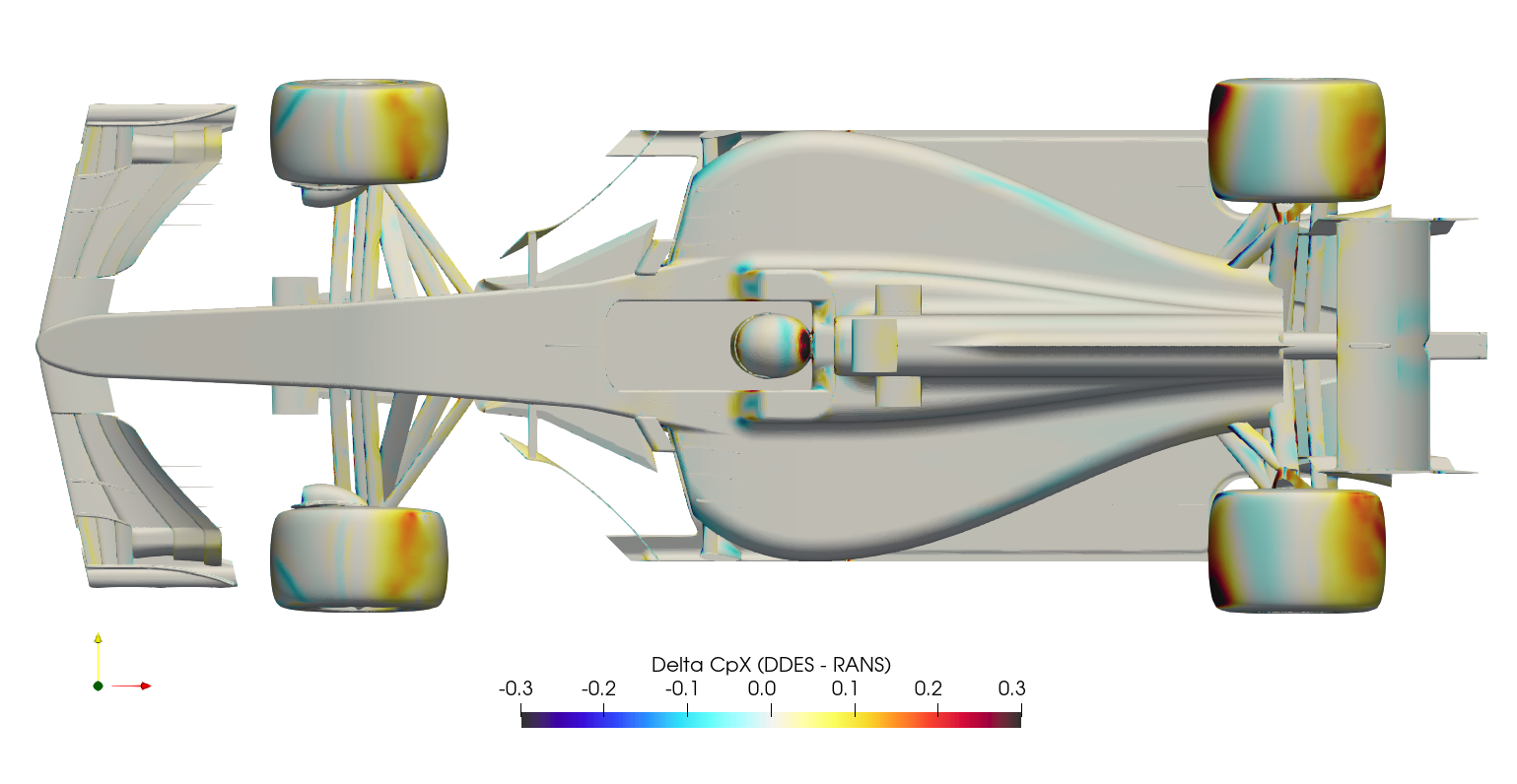
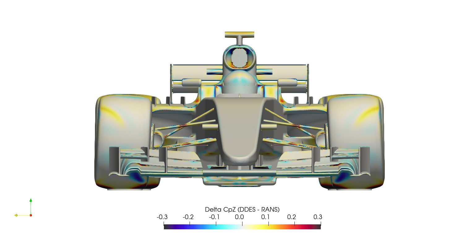
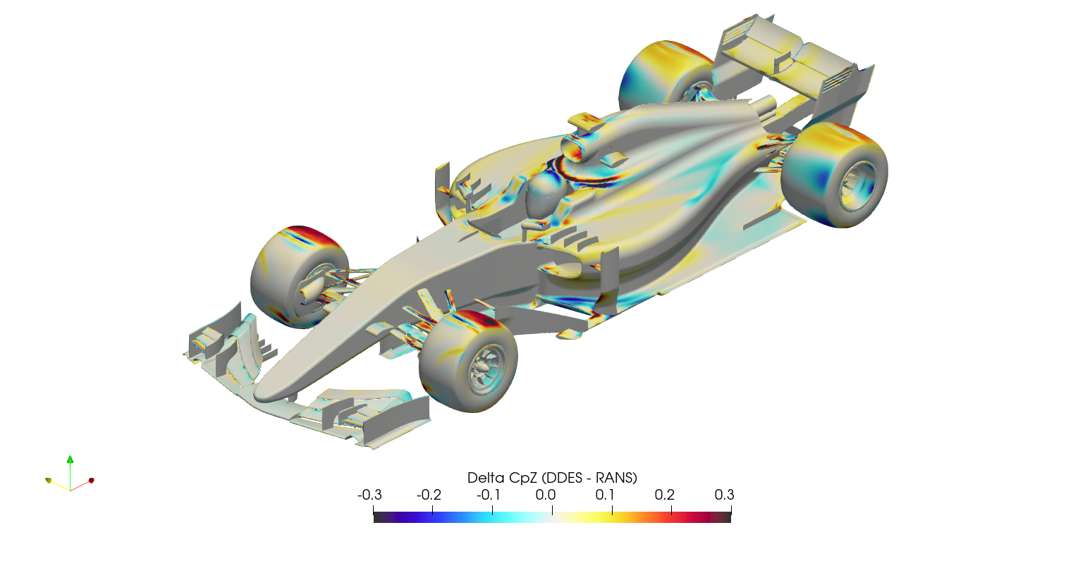
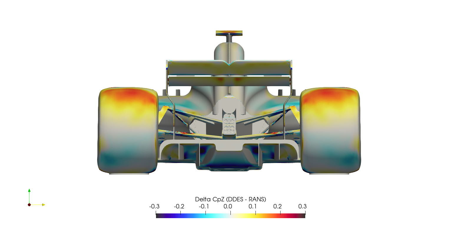
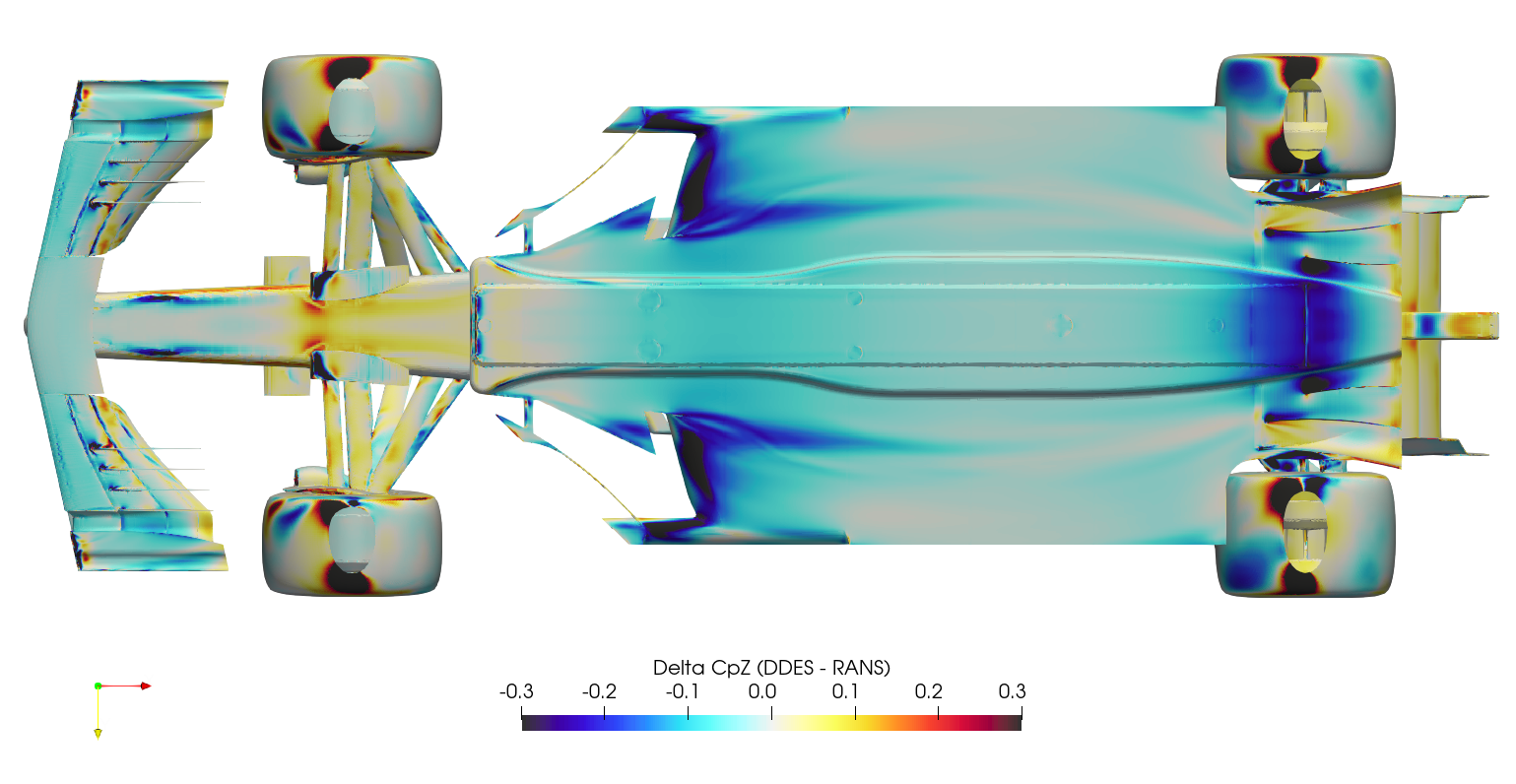
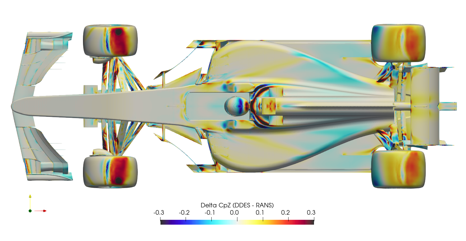
The transient DDES solution resolves the flow parameters through time, capturing the unsteady behavior. The result of this additional resolution can be seen in the large difference in drag prediction for the front and rear wheels. The wheels are bluff-bodies with a large separated region downstream. The RANS solution struggles to resolve this region, which results in an overprediction of downstream pressure and hence reduced drag on the wheels. Another significant difference is the underfloor pressure distribution. The delta surface plots (following section) show significantly lower pressures on the underfloor for the DDES case, highlighted in the CpZ underfloor plot. The effect of this reduced underfloor pressure can be seen in the lift accumulation plot and the component lift breakdown.
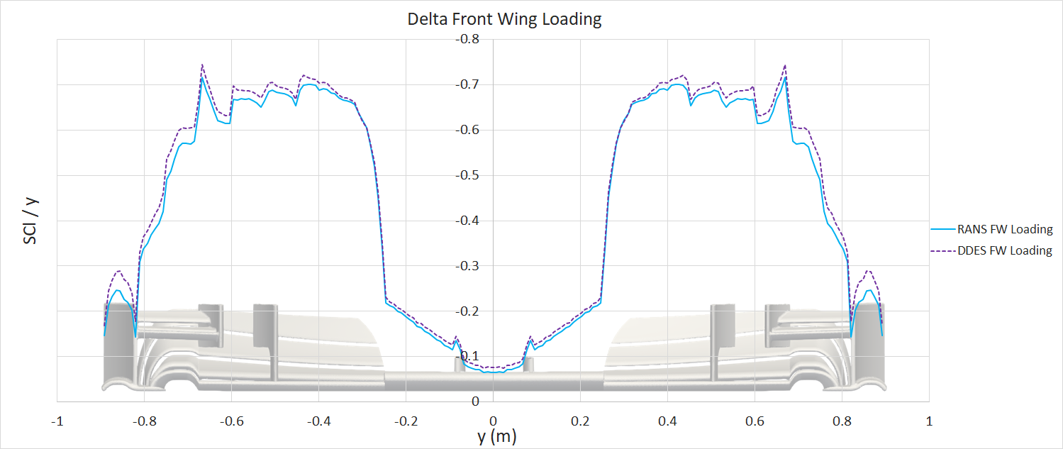
The front and rear wing are investigated further, in isolation. The code used to extract the force-accumulation data has been modified to sweep across the isolated wings in the y-direction, producing spanwise loading data. This force data has been normalised by the freestream dynamic pressure multiplied by the discretised section thickness. The data has been reflected in the plot, to account for the other half of the car.
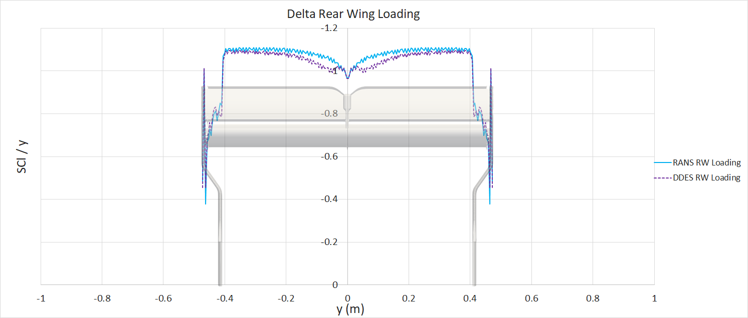
From the component force breakdown, the front wing generates more downforce in the DDES case. Whereas, the rear wing generates more downforce in the RANS case. The wing loading plots highlight the areas of the wings producing more/less downforce.
For the front wing, the area of the wing producing the largest downforce, in both cases, is between y300 (y=300mm) and y700. The DDES case predicts larger downforce across the entire span, but overall has a very similar load distribution to the RANS case.
For the rear wind, there is less downforce generated between y0 and y400 for the DDES case. This could be caused by a number of factors. The gurney flap on the upper element may cause an unsteady wake, which may not be properly resolved in the RANS case, compared to the DDES case. The symmetry plane may also be influencing the DDES result, by constraining the flow in the xz direction; there may be non-physical flow features forming where the wing meets the symmetry plane. Finally, the oncoming flow may be different. The wing sits in the wake of the body/roll-structure. The rear wing has reduced onset flow quality in the DDES case, resulting in slightly lower downforce potential (see next paragraph).
As previously mentioned, the flow field around the vehicle changes between the RANS and DDES case. Flow total pressure is often used as measure of flow energy/potential. A gif is presented showing a sweeping x-slice, displaying the iteration-averaged/time-average total pressure coefficient over the car, for both cases. The slice has been clipped to only contain CpT values less than 1. As previously discussed, the rear wing produced less downforce between y0 and y400 in the DDES case. The gif shows a slightly larger region of lower energy flow hitting the center of the rear wing, when compared to the RANS case.
\[ CpT = \frac{static\: pressure\:+\:\frac{1}{2}\:ρ\:U^2}{\frac{1}{2}\:ρ\:U_\infty^2} \]
Note - the following gif may require desktop viewing, and may require some time to load.

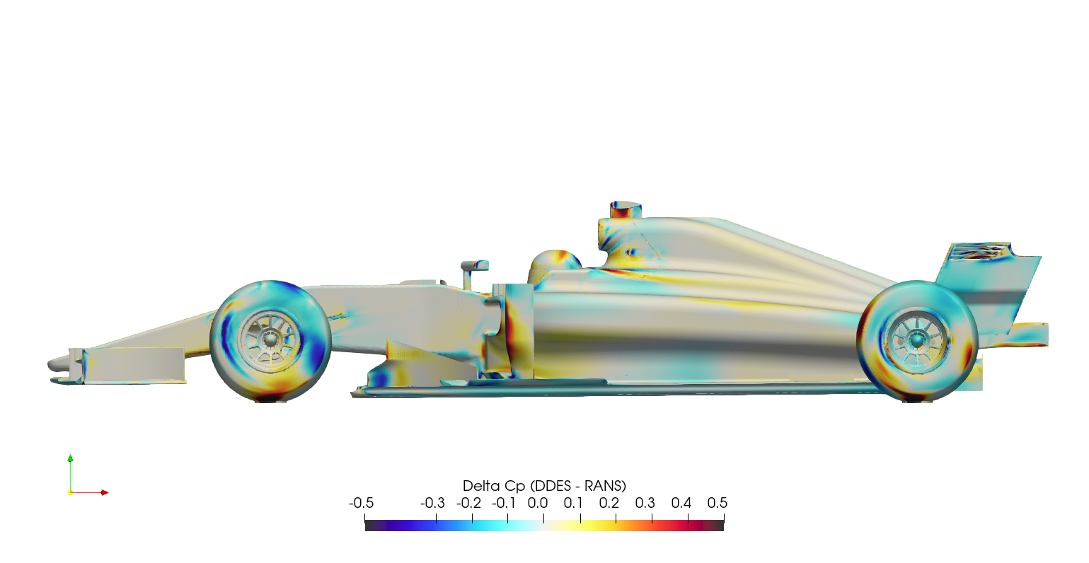
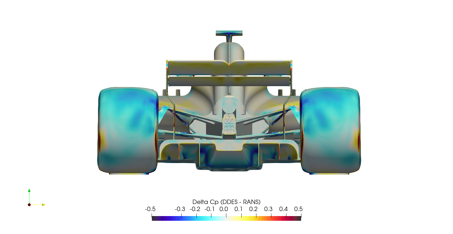
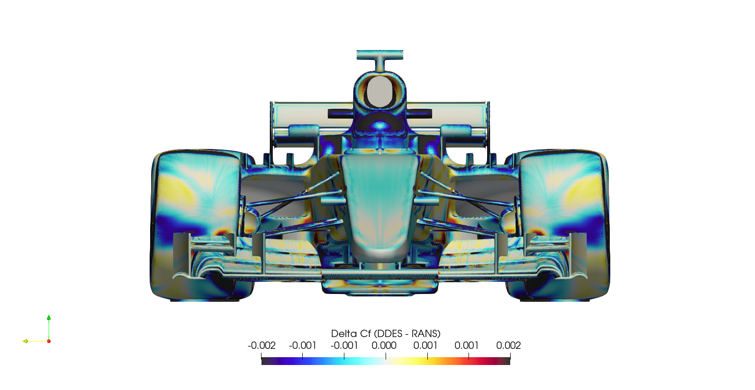
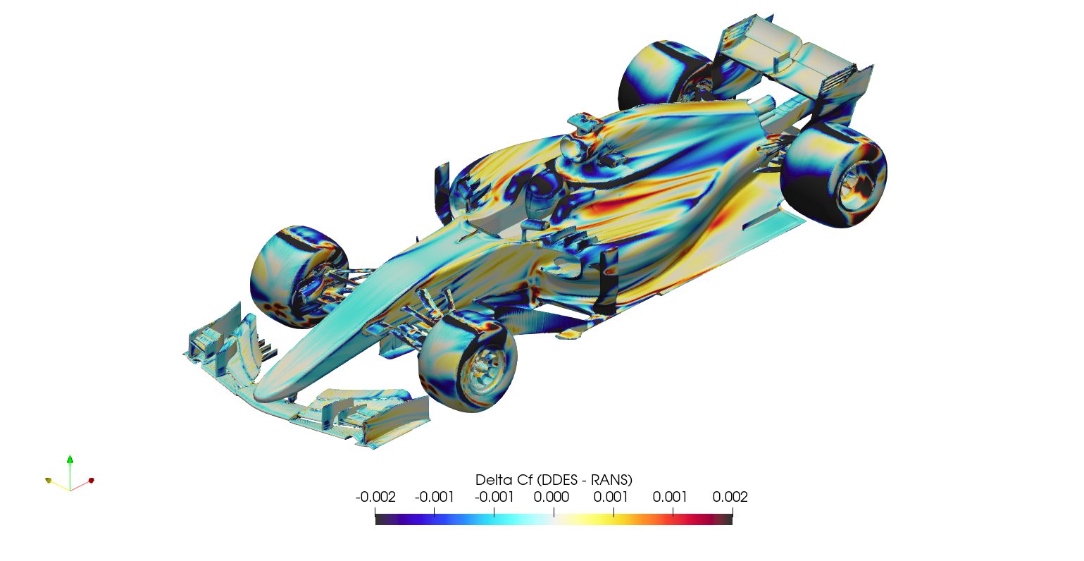
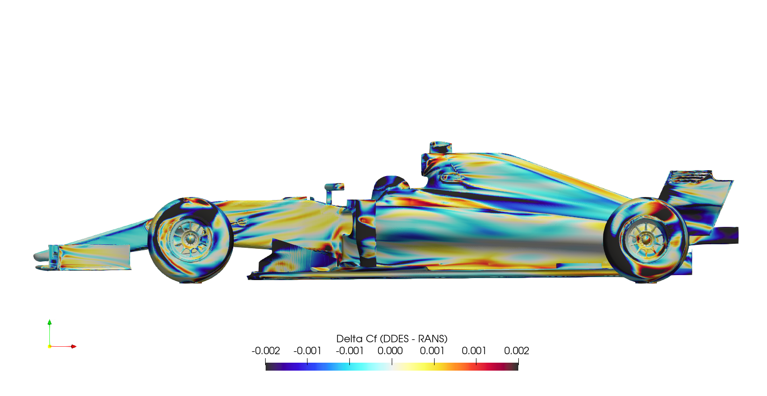
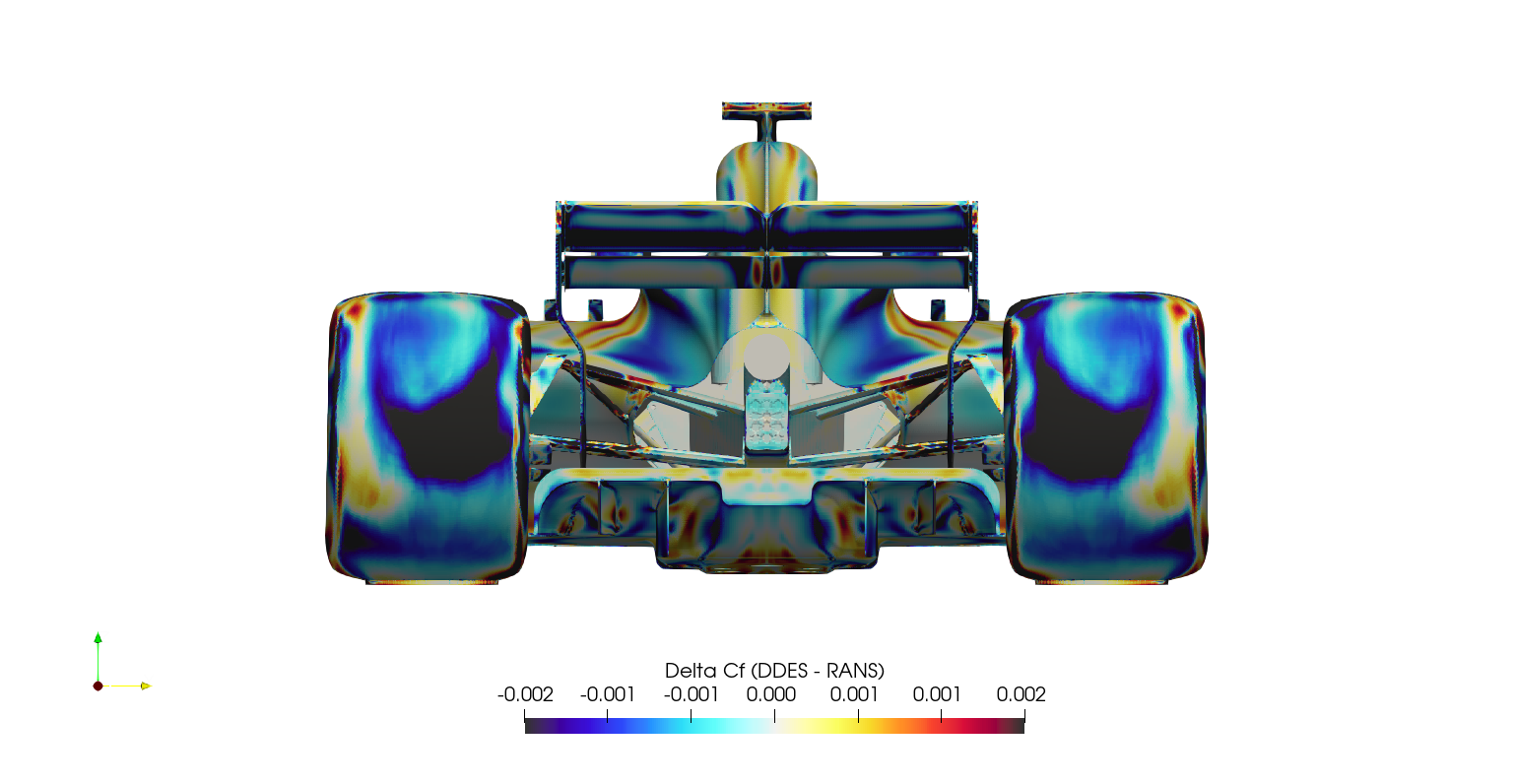
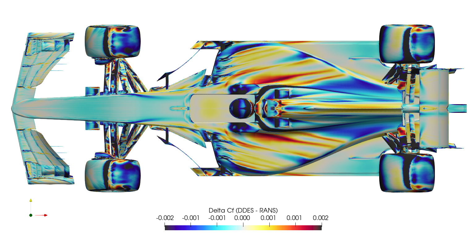
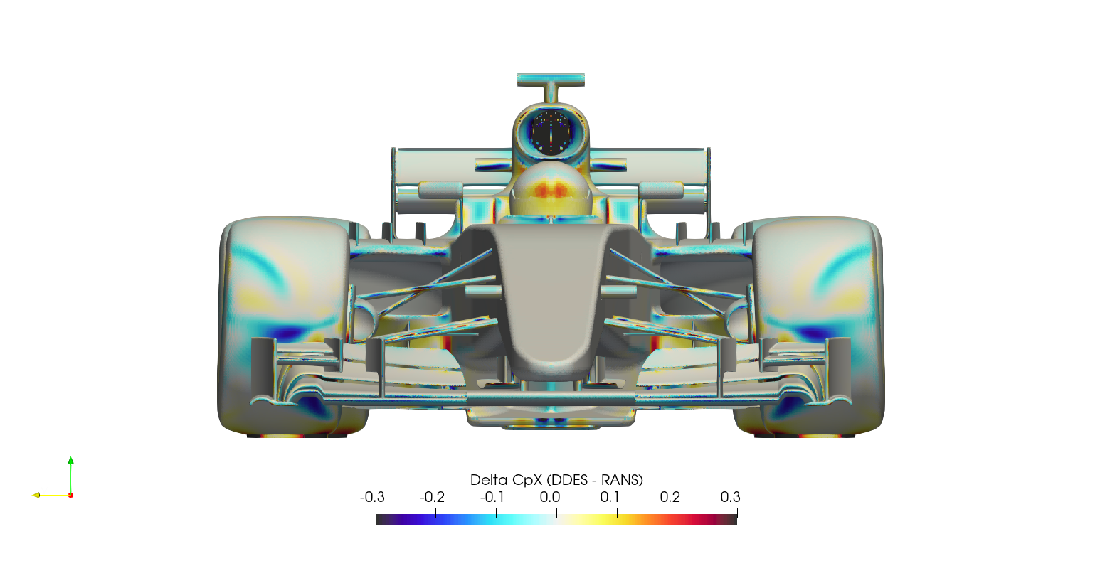
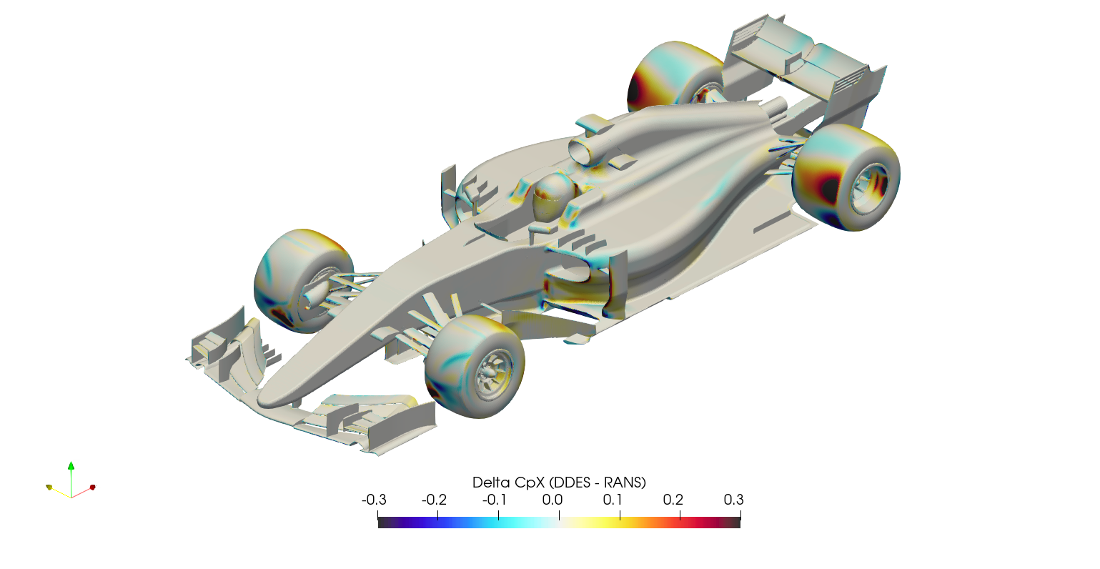
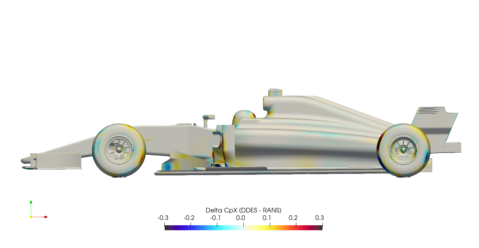
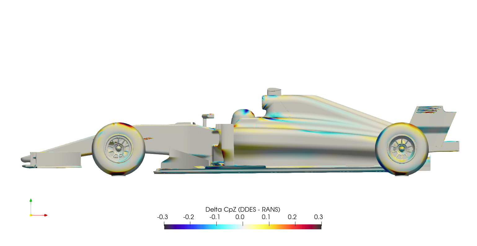
Steady-state RANS vs. Transient DDES - Delta Post-processing
It's difficult to compare surface plots between the two cases directly, this creates a 'spot the difference' situation. Instead, it's easier to subtract the RANS surface variables from the DDES surface variables at each location, and plot the result as a 'delta'. This is normally a difficult operation, since there will usually be slight differences in geometry/mesh, meaning the variables of one case have to be mapped/interpolated onto the surface from the other case. Fortunately in this case, the geometry/mesh was identical between cases, meaning the surface variables from the RANS case could be mapped to the DDES case directly through manipulation of the ensight files. Once the field variables for both the RANS and the DDES were stored within a single ensight file, the calculation was executed in paraview, subtracting the RANS variables from the DDES variables, and the series of images below were created.

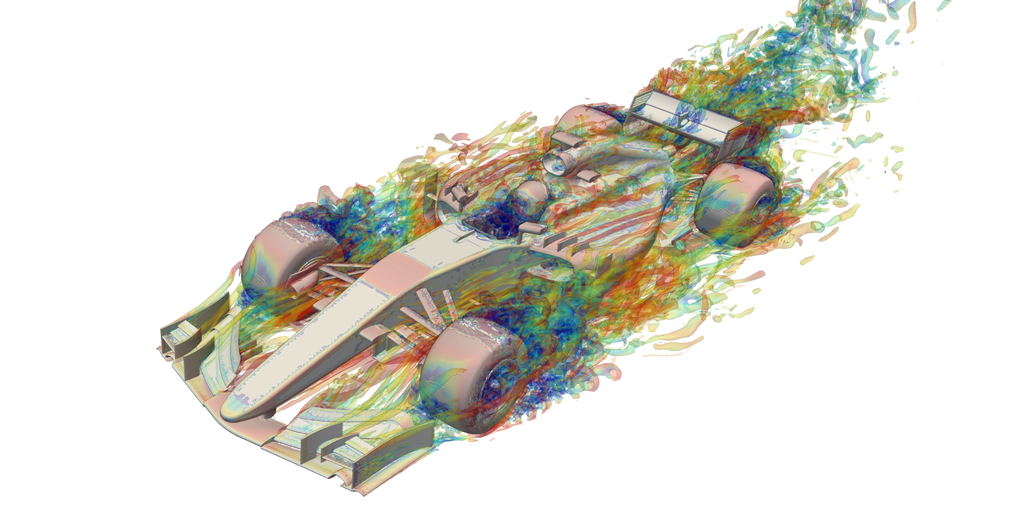
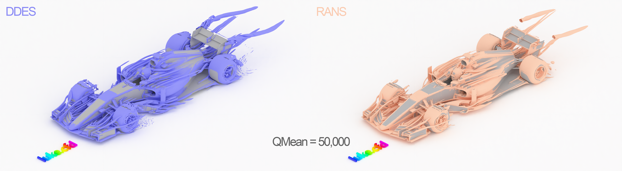
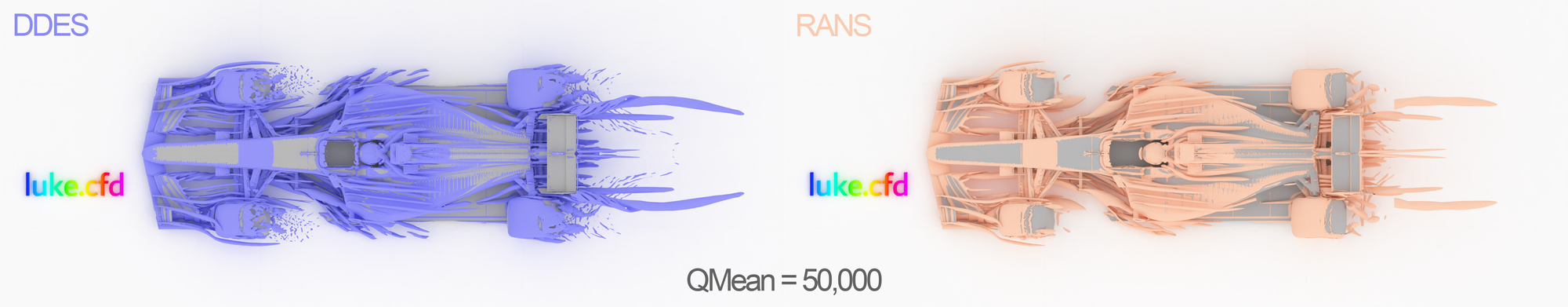
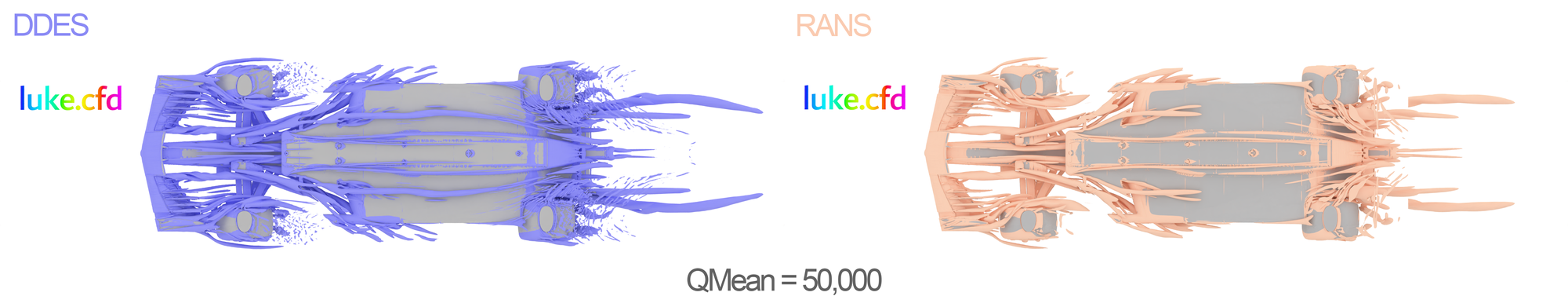
The production of downforce is closely linked to to the management of vortices around the car. The Q-criterion is a scalar used to highlight these structures around the car, where the vorticity magnitude is greater than the magnitude of the rate of strain. The plots below show QMean=50,000 isosurfaces, for both the DDES case and the RANS case.
The isosurfaces were generated directly in OpenFOAM using a functionObject. Unfortunately the isosurface for the RANS case appears to have not been generated correctly at the rear wing, where the mesh changes cell size.
Finally, a render of time varying CpT is presented on the y0 and y400 planes for the DDES case. The opacity of the car is reduced for the y400 slice to show the flow into the side pod and through the radiator.
Conclusions / Further Work
The main objectives and aims of this investigation have been met. A process has been created in native OpenFOAM which allows for a crude numerical assessment of a Formula 1 car.
The process could likely be improved dramatically with more computational resource, which would allow for larger meshes, mesh dependency studies, full car cases, yaw angles, further testing of turbulence modelling and performance maps at various ride heights/rake angles.
The results of this study are not correct, but provide an indication of the forces acting on the car and it's front balance. The SCl number for the car is significantly lower than that of a fully developed Formula 1 car.
It would be interesting to do some further investigations if time permits. For example testing different turbulence models, ride heights, sensitivities to solver settings and courant numbers.
It would be very interesting to test one of the 2022 cars, to see the effect of the underfloor and how it changes the shape of the drag/lift accumulation plots. It would also be interesting to look at the flow quality downstream and compare back to this study. Hopefully one day another high quality open-source model will be developed!